Langley Research Center

Turbulence Modeling Resource

K-e-zeta-f Turbulence Model

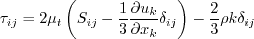
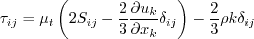
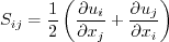
This web page gives detailed information on the equations for the three-equation (plus elliptic relaxation equation, for a total of four equations) k-e-zeta-f turbulence closure. All forms of the model given on this page are linear eddy viscosity models. Linear models use the Boussinesq assumption for the constitutive relation:

$\tau_{ij} = 2 \mu_t \left(S_{ij} - \frac{1}{3} \frac{\partial u_k}{\partial x_k} \delta_{ij} \right) - \frac{2}{3} \rho k \delta_{ij}$

Unless otherwise stated, for compressible flow with heat transfer this model is implemented as described on the page Implementing Turbulence Models into the Compressible RANS Equations, with perfect gas assumed and Pr = 0.72, Pr_t = 0.90, and Sutherland's law for dynamic viscosity.

Return to: Turbulence Modeling Resource Home Page

K-e-zeta-f2004 Model (k-e-zeta-f2004)

This model's references are:

Hanjalic, K., Popovac, M., Hadziabdic, M., "A Robust Near-Wall Elliptic-Relaxation Eddy-Viscosity Turbulence Model for CFD," International Journal of Heat and Fluid Flow, Vol. 25, 2004, pp. 1047-1051, https://doi.org/10.1016/j.ijheatfluidflow.2004.07.005.
Popovac, M., Hanjalic, K., "Compound Wall Treatment for RANS Computation of Complex Turbulent Flows and Heat Transfer," Flow, Turbulence, and Combustion, Vol. 78, 2007, pp. 177-202, https://doi.org/10.1007/s10494-006-9067-x.

Note the latter reference has a typo in the equation for the time scale, T.

This model is based on original ideas of Durbin (see, e.g., the k-e-v²-f model as described in AIAA Journal, Vol. 33, No. 4, 1995, pp. 659-664, https://doi.org/10.2514/3.12628). Note that $\zeta = v^2 / k$ . The k-e-zeta-f2004 model is also described online at:

CFD Online, "Zeta-f model," http://www.cfd-online.com/Wiki/Zeta-f_model.

This model (written in conservation form) is given by the following:

$\frac{\partial \rho k}{\partial t} + \frac{\partial (\rho u_j k)}{\partial x_j} = P - \rho \varepsilon + \frac{\partial}{\partial x_j} \left[ \left( \mu + \frac{\mu_t}{\sigma_k} \right) \frac{\partial k}{\partial x_j} \right]$

$\frac{\partial \rho \varepsilon}{\partial t} + \frac{\partial (\rho u_j \varepsilon)}{\partial x_j} = \frac{C_{\varepsilon 1} P - C_{\varepsilon 2} \rho \varepsilon}{T} + \frac{\partial}{\partial x_j} \left[ \left( \mu + \frac{\mu_t}{\sigma_{\varepsilon}} \right) \frac{\partial \varepsilon}{\partial x_j} \right]$

$\frac{\partial \rho \zeta}{\partial t} + \frac{\partial (\rho u_j \zeta)}{\partial x_j} = \rho f - \frac{\zeta}{k}P + \frac{\partial}{\partial x_j} \left[ \left( \mu + \frac{\mu_t}{\sigma_{\zeta}} \right) \frac{\partial \zeta}{\partial x_j} \right]$

Non-locality is represented by an elliptic relaxation equation for f:

$L^2\nabla^2 f - f = L^2\frac{\partial}{\partial x_j}\left(\frac{\partial f}{\partial x_j}\right) -f = \frac{1}{T} \left(C_1 - 1 + C_2' \frac{P}{\rho \varepsilon} \right) \left(\zeta - \frac{2}{3} \right)$

where

$P = \tau_{ij} \frac{\partial u_i}{\partial x_j}$

$\tau_{ij} = \mu_t \left(2S_{ij} - \frac{2}{3} \frac{\partial u_k}{\partial x_k} \delta_{ij} \right) - \frac{2}{3} \rho k \delta_{ij}$

$S_{ij} = \frac{1}{2} \left( \frac{\partial u_i}{\partial x_j} + \frac{\partial u_j}{\partial x_i} \right)$

Note for incompressible flows, the production term exactly becomes:

$P = \mu_t S^2$

(which is often taken as a good approximation except for very high Mach numbers; see Notes on Running the Cases with CFD, note 4). Here, $S=\sqrt{2 S_{ij} S_{ij}}$ .

The turbulent eddy viscosity is computed from:

$\mu_t = \rho C_{\mu} \zeta k T$

The time scale and length scale are computed from:

$T = {\rm max} \left[ {\rm min} \left( \frac{k}{\varepsilon}, \frac{0.6}{\sqrt{6} C_{\mu} |S| \zeta} \right), C_T \left( \frac{\nu}{\varepsilon} \right)^{1/2} \right]$

$L = C_L {\rm max} \left[ {\rm min} \left( \frac{k^{3/2}}{\varepsilon}, \frac{k^{1/2}}{\sqrt{6} C_{\mu} |S| \zeta} \right), C_{\eta} \left( \frac{\nu^3}{\varepsilon} \right)^{1/4} \right]$

The closure coefficients are:

$C_{\mu} = 0.22$ $\sigma_k = 1.0$

$\sigma_{\varepsilon} = 1.3$ $\sigma_{\zeta} = 1.2$

$C_{\varepsilon 1} = 1.4[1+(0.012/\zeta)]$ $C_{\varepsilon 2} = 1.9$

$C_1 = 1.4$ $C_2' = 0.65$

$C_T = 6$ $C_L = 0.36$ $C_{\eta} = 85$

There are no specific farfield boundary conditions recommended for this model.

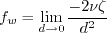
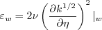
At the wall, the boundary conditions are:

$k_w = 0$

$\varepsilon_w = \lim_{d\to0}{\frac{2 \nu k}{d^2}}$

$\zeta_w = 0$

$f_w = \lim_{d\to0}{\frac{-2 \nu \zeta}{d^2}}$

with d = distance to the wall, and numerical implementation details for the limit terms are unspecified in the original papers. As implied in Kalitzin (AIAA 99-3780), a typical implementation for these terms might be:

$\varepsilon_w = \frac{2 \nu_1 k_1}{d_1^2}$

$f_w = -\frac{2 \nu_1 \zeta_1}{d_1^2}$

where the subscript "1" indicates the value at the first interior grid point or cell center above the wall. Note that another common wall BC used for $\varepsilon$ is:

$\varepsilon_w = 2 \nu \left( \frac{\partial k^{1/2}}{\partial \eta} \right)^2 |_w$

where $\eta$ is the direction normal to the wall (see Hanjalic and Launder, Modelling Turbulence in Engineering and the Environment, Cambridge University Press, 2011, section 6.2).

(Although not described in detail here, it is also possible to manipulate the $\varepsilon$ and f equations so that $\tilde \varepsilon_w = 0$ and $\tilde f_w = 0$ , using

$\tilde \varepsilon = \varepsilon - \frac{2 \nu k}{d^2}$

$\tilde f = f + \frac{2 \nu \zeta}{d^2}$

See Hanjalic and Launder, Modelling Turbulence in Engineering and the Environment, Cambridge University Press, 2011, sections 6.2 and 7.4.)

Return to: Turbulence Modeling Resource Home Page

Privacy Act Statement

Accessibility Statement

Responsible NASA Official: Ethan Vogel
Page Curator: Clark Pederson
Last Updated: 11/08/2021