Langley Research Center

Turbulence Modeling Resource

K-kL Turbulence Model

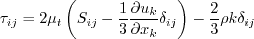
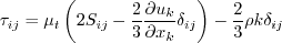
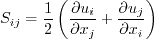
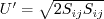
This web page gives detailed information on the equations for various forms of the k-kL turbulence model. All forms of the model given on this page are linear eddy viscosity models. Linear models use the Boussinesq assumption for the constitutive relation:

$\tau_{ij} = 2 \mu_t \left(S_{ij} - \frac{1}{3} \frac{\partial u_k}{\partial x_k} \delta_{ij} \right) - \frac{2}{3} \rho k \delta_{ij}$

Unless otherwise stated, for compressible flow with heat transfer this model is implemented as described on the page Implementing Turbulence Models into the Compressible RANS Equations, with perfect gas assumed and Pr = 0.72, Pr_t = 0.90, and Sutherland's law for dynamic viscosity.

Return to: Turbulence Modeling Resource Home Page

K-kL Model from Menter/Egorov and Abdol-Hamid (k-kL-MEAH2015) and (k-kL-MEAH2015m)

This version of k-kL is an update of k-kL-MEAH2013. There are only a few relatively minor differences from the 2013 version. The reference is:

Abdol-Hamid, K. S., Carlson, J.-R., and Rumsey, C. L., "Verification and Validation of the k-kL Turbulence Model in FUN3D and CFL3D Codes," AIAA Paper 2016-3941, June 2016, https://doi.org/10.2514/6.2016-3941.
Abdol-Hamid, K. S., Carlson, J.-R., and Rumsey, C. L., "Verification and Validation of the k-kL Turbulence Model in FUN3D and CFL3D Codes," NASA/TM-2015-218968, November 2015, https://ntrs.nasa.gov/citations/20160000768.

The two-equation model (written in conservation form) is given by the following:

$\frac{\partial (\rho k)}{\partial t} + \frac{\partial (\rho u_j k)}{\partial x_j} = \cal P - C_{\mu}^{3/4}\rho \frac{k^{5/2}}{(kL)} - 2 \mu \frac{k}{d^2} + \frac{\partial}{\partial x_j} \left[\left(\mu + \sigma_k \mu_t \right)\frac{\partial k}{\partial x_j}\right]$

$\frac{\partial (\rho (kL))}{\partial t} + \frac{\partial (\rho u_j (kL))}{\partial x_j} = C_{\phi 1}\frac{(kL)}{k} \cal P - C_{\phi 2} \rho k^{3/2} - 6 \mu \frac{(kL)}{d^2}f_{\phi} + \frac{\partial}{\partial x_j} \left[ \left( \mu + \sigma_{\phi} \mu_t \right) \frac{\partial (kL)}{\partial x_j} \right]$

$P = \tau_{ij} \frac{\partial u_i}{\partial x_j}$

$\tau_{ij} = \mu_t \left(2S_{ij} - \frac{2}{3} \frac{\partial u_k}{\partial x_k} \delta_{ij} \right) - \frac{2}{3} \rho k \delta_{ij}$

$S_{ij} = \frac{1}{2} \left( \frac{\partial u_i}{\partial x_j} + \frac{\partial u_j}{\partial x_i} \right)$

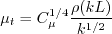
and the turbulent eddy viscosity is computed from:

$\mu_t = C_{\mu}^{1/4} \frac{\rho (kL)}{k^{1/2}}$

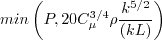
Different from k-kL-MEAH-2013, the production term P in both the k and kL equations is limited, and gets replaced by:

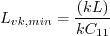
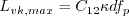
$min\left(P, 20 C_{\mu}^{3/4}\rho \frac{k^{5/2}}{(kL)}\right)$

The functions are:

$C_{\phi 1} = \left[ \zeta_1 - \zeta_2 \left( \frac{(kL)}{k L_{vk}} \right)^2 \right]$

$C_{\phi 2} = \zeta_3$

$f_{\phi} = \frac{1+C_{d1} \xi}{1 + \xi^4}$

where

$L_{vk} = \kappa \left| \frac{U'}{U''} \right|$

$U' = \sqrt{2 S_{ij} S_{ij}}$

$U'' = \sqrt{ \left(\frac{\partial^2u}{\partial x^2} + \frac{\partial^2u}{\partial y^2} + \frac{\partial^2u}{\partial z^2} \right)^2 + \left(\frac{\partial^2v}{\partial x^2} + \frac{\partial^2v}{\partial y^2} + \frac{\partial^2v}{\partial z^2} \right)^2 + \left(\frac{\partial^2w}{\partial x^2} + \frac{\partial^2w}{\partial y^2} + \frac{\partial^2w}{\partial z^2} \right)^2 }$

$\xi = \frac{\rho d \sqrt{0.3 k}}{20 \mu}$

and $\rho$ is the density, $\mu$ is the molecular dynamic viscosity, and d is the distance from the field point to the nearest wall. Note that if U' = U'' = 0, then the (kL) production term should be identically zero.

A limiter (different from k-kL-MEAH-2013) is applied on $L_{vk}$ :

$L_{vk,min} \leq L_{vk} \leq L_{vk,max}$

with

$L_{vk,min}=\frac{(kL)}{k C_{11}}$

$L_{vk,max}=C_{12} \kappa d f_p$

$f_p=min\left[ max\left(\frac{\cal P}{\left(C_{\mu}^{3/4} \rho k^{5/2}/(kL) \right)} , 0.5 \right) , 1.0 \right]$

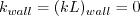
The boundary conditions for the two turbulence variables k and (kL) at walls are:

$k_{wall} = (kL)_{wall} = 0$

Note: the zero BC for k can cause a divide-by-zero if one tries to compute turbulent eddy viscosity at the wall (with equation given earlier). However, the turbulent eddy viscosity at the wall is identically zero, so this numerical issue can be bypassed.

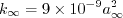
Recommended farfield boundary conditions for most applications are:

$k_{\infty} = 9 \times 10^{-9} a_{\infty}^2$

$(kL)_{\infty} = 1.5589 \times 10^{-6} \mu_{\infty}a_{\infty}/\rho_{\infty}$

where a represents the speed of sound.

The constants are:

$\zeta_1 = 1.2$ $\zeta_2 = 0.97$ $\zeta_3 = 0.13$

$\sigma_k = 1.0$ $\sigma_{\phi} = 1.0$

$\kappa = 0.41$ $C_{\mu} = 0.09$

$C_{11} = 10.0$ $C_{12} = 1.3$ $C_{d1} = 4.7$

Note: the $(2/3) \overline \rho k \delta_{ij}$ term in the Boussinesq approximation for tau_ij is sometimes ignored in the momentum and energy equations. Similarly, the production term in two-equation turbulence models is often approximated by P = mu_t S². This expression is exact for incompressible flows and is typically considered a very good approximation, except perhaps for very high Mach number flows (see items 4 and 7 on the page Notes on Running the Cases with CFD, and the Implementing Turbulence Models into the Compressible RANS Equations page). When the $(2/3) \overline \rho k \delta_{ij}$ term is ignored in tau_ij in the momentum and energy equations and the production term is approximated by P = mu_t S², a modified naming convention should be employed: (k-kL-MEAH2015m).

K-kL Model from Menter/Egorov and Abdol-Hamid (k-kL-MEAH2013) and (k-kL-MEAH2013m)

This version of k-kL derives from three references:

Menter, F. R. and Egorov, Y., "The Scale-Adaptive Simulation Method for Unsteady Turbulent Flow Predictions. Part 1: Theory and Model Description," Flow, Turbulence, and Combustion, Vol. 85, 2010, pp. 113-138, https://doi.org/10.1007/s10494-010-9264-5.
Abdol-Hamid, K. S., "Assessmants of k-kL Turbulence Model Based on Menter's Modification to Rotta's Two-Equation Model," International Journal of Aerospace Engineering, Vol. 2015, Article ID 987682, http://doi.org/10.1155/2015/987682.
Abdol-Hamid, K. S., "Assessments of a Turbulence Model Based on Menter's Modification to Rotta's Two-Equation Model," AIAA Paper 2013-0341, January 2013, https://doi.org/10.2514/6.2013-341.

Although the first reference introduced this method, its focus was primarily on a hybrid model of different form; the second reference fine-tuned the k-kL version given below. Note that there is some missing information in the second and third references: (1) kappa should be given as 0.41, and (2) C_d1 should be given as 4.7 for k-kL. In the third reference, the following typos are also noted: (1) eqn 4 should have (p1-2) exponent rather than (p1-1.5), and (2) parentheses are missing in the diffusion terms. These have been corrected below. The compressibility correction factor from the second and third references is not included here.

The two-equation model (written in conservation form) is given by the following:

$P = \tau_{ij} \frac{\partial u_i}{\partial x_j}$

$\tau_{ij} = \mu_t \left(2S_{ij} - \frac{2}{3} \frac{\partial u_k}{\partial x_k} \delta_{ij} \right) - \frac{2}{3} \rho k \delta_{ij}$

$S_{ij} = \frac{1}{2} \left( \frac{\partial u_i}{\partial x_j} + \frac{\partial u_j}{\partial x_i} \right)$

and the turbulent eddy viscosity is computed from:

$\mu_t = C_{\mu}^{1/4} \frac{\rho (kL)}{k^{1/2}}$

The functions are:

$C_{\phi 1} = \left[ \zeta_1 - \zeta_2 \left( \frac{(kL)}{k L_{vk}} \right)^2 \right]$

$C_{\phi 2} = \zeta_3$

$f_{\phi} = \frac{1+C_{d1} \xi}{1 + \xi^4}$

where

$L_{vk} = \kappa \left| \frac{U'}{U''} \right|$

$U' = \sqrt{2 S_{ij} S_{ij}}$

$\xi = \frac{\rho d \sqrt{0.3 k}}{20 \mu}$

A limiter is applied on $L_{vk}$ :

$\frac{(kL)}{k C_{11}} < L_{vk} < C_{12} \kappa d \left[ \frac{\cal P}{\left(C_{\mu}^{3/4} \rho k^{5/2}/(kL) \right)} \right]$

The boundary conditions for the two turbulence variables k and (kL) at walls are:

$k_{wall} = (kL)_{wall} = 0$

No specific farfield boundary conditions have been recommended for this model.

The constants are:

$\zeta_1 = 1.2$ $\zeta_2 = 0.97$ $\zeta_3 = 0.13$

$\sigma_k = 1.0$ $\sigma_{\phi} = 1.0$

$\kappa = 0.41$ $C_{\mu} = 0.09$

$C_{11} = 10.0$ $C_{12} = 1.3$ $C_{d1} = 4.7$

When the $(2/3) \overline \rho k \delta_{ij}$ term is ignored in tau_ij in the momentum and energy equations and the production term is approximated by P = mu_t S², a modified naming convention should be used: (k-kL-MEAH2013m).

Return to: Turbulence Modeling Resource Home Page

Recent significant updates:
03/24/2021 - clarifications on use of "m" designation when P=mu_t S² and k term ignored in momentum and energy equations
03/27/2017 - mention how to handle turbulent eddy visocity at walls
06/30/2015 - mention Pr, Pr_t, and Sutherland's law
05/14/2015 - added journal article reference

Privacy Act Statement

Accessibility Statement

Responsible NASA Official: Ethan Vogel
Page Curator: Clark Pederson
Last Updated: 11/08/2021