
 |
Langley Research CenterTurbulence Modeling Resource |
Transitional SSG/LRR Reynolds Stress Model
This web page gives detailed information on the equations for various forms of the transitional SSG/LRR Reynolds stress model,
which is a blend between Langtry-Menter γ-Reθt equations and full second-moment Reynolds stress equations. Full second-moment Reynolds stress models are very different from simpler one and two-equation
linear/nonlinear models, in that the latter use a constitutive relation giving the Reynolds stresses Unless otherwise stated, for compressible flow with heat transfer this model is implemented as described on the page
Implementing Turbulence Models into the Compressible RANS Equations, with perfect gas
assumed and Pr = 0.72, Prt = 0.90, and Sutherland's law for dynamic viscosity.
Return to: Turbulence Modeling Resource Home Page Transitional SSG/LRR Reynolds Stress Model
(SSG/LRR-trans)
This model is developed by coupling of the SSG/LRR-w2012-SD full turbulence model with the Langtry-Menter γ-Reθt model. The primary reference for the implementation of the 9-equation transitional RSM is:
Note that the SSG/LRR-ω model almost shares the same length-scale determining equation as the Menter’s k-ω SST model, except the production term. The production of ω in Langtry-Menter’s 4-equation model is linear to the square of the mean strain rate.
In contrast to the ω-based RSM coupling with γ-Reθt, the ω production does not vanish in the fully laminar region. Along with this, an inverse-ω scale variable(
The λ equals 0 strictly on the viscous wall and so avoids the invalidity of generation term upstream the transition onset. Based on this, the model is given by the following:
 in terms of other tensors via some assumed relation (such as Boussinesq's hypothesis). On
the other hand, full second-moment Reynolds stress models compute each of the 6 Reynolds stresses directly (the Reynolds stress tensor is symmetric so there are 6 independent terms). Each Reynolds stress
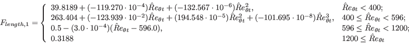
has its own transport equation. There is also a seventh transport equation for the lengthscale-determining variable.
in terms of other tensors via some assumed relation (such as Boussinesq's hypothesis). On
the other hand, full second-moment Reynolds stress models compute each of the 6 Reynolds stresses directly (the Reynolds stress tensor is symmetric so there are 6 independent terms). Each Reynolds stress
has its own transport equation. There is also a seventh transport equation for the lengthscale-determining variable.
![]() )
is recommended by:
)
is recommended by:
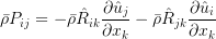
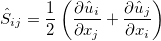
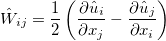
The source terms in Reynolds stress equations are defined as:
![\begin{gathered}
\frac{\partial\left(\bar{\boldsymbol{\rho}}\hat{R}_{ij}\right)}{\partial t}+\frac{\partial\left(\bar{\boldsymbol{\rho}}\hat{u}_k\hat{R}_{ij}\right)}{\partial x_k}=\bar{\boldsymbol{\rho}}P_{ij}+\bar{\boldsymbol{\rho}}\Pi_{ij}-\bar{\boldsymbol{\rho}}\varepsilon_{ij}+\bar{\boldsymbol{\rho}}D_{ij} \\
\frac{\partial(\bar{\rho}\lambda)}{\partial t}+\frac{\partial(\bar{\rho}\hat{u}_k\lambda)}{\partial x_k}=\bar{\rho}P_\lambda-\bar{\rho}\varepsilon_\lambda+\bar{\rho}D_\lambda+\bar{\rho}C_{D\lambda}+\bar{\rho}G_\lambda \\
\frac{\partial(\bar{\boldsymbol{\rho}}\boldsymbol{\gamma})}{\partial t}+\frac{\partial(\bar{\boldsymbol{\rho}}\hat{\boldsymbol{u}}_j\boldsymbol{\gamma})}{\partial x_j}=P_{\boldsymbol{\gamma}}-E_{\boldsymbol{\gamma}}+\frac{\partial}{\partial x_j}\left[\left(\boldsymbol{\mu}+\frac{\boldsymbol{\mu}_t}{\boldsymbol{\sigma}_f}\right)\frac{\partial\boldsymbol{\gamma}}{\partial x_j}\right] \\
\frac{\partial\left(\bar{\boldsymbol{\rho}}\tilde{R}e_{\boldsymbol{\theta}t}\right)}{\partial t}+\frac{\partial\left(\bar{\boldsymbol{\rho}}\hat{u}_{j}\tilde{R}e_{\boldsymbol{\theta}t}\right)}{\partial x_{j}}=P_{\boldsymbol{\theta}t}+\frac{\partial}{\partial x_{j}}\left[\boldsymbol{\sigma}_{\boldsymbol{\theta}t}\left(\boldsymbol{\mu}+\boldsymbol{\mu}_{t}\right)\frac{\partial\tilde{R}e_{\boldsymbol{\theta}t}}{\partial x_{j}}\right]
\end{gathered}](./Transitional_SSGLRR_Reynolds_Stress_Model_files/Rij.png )

![\bar{\rho}D_{ij}=\frac{\partial}{\partial x_k}\left[\left(\mu+\frac{D}{C_\mu}\mu_t\right)\frac{\partial\hat{R}_{ij}}{\partial x_k}\right]](./Transitional_SSGLRR_Reynolds_Stress_Model_files/Dij.png)
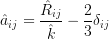
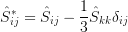
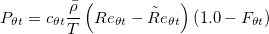
The dissipation rate as well as turbulence viscosity are as follows:

 at the solid wall and in the far-field are given as:
 , the hat represents the Favre average,
  ,
,  is the non-weighted averaging density,
  is the molecular dynamic viscosity,
  is the distance from the field point to the nearest wall,
 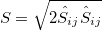 is the strain rate magnitude, and
 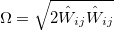 is the vorticity magnitude, with
The source terms for the  equation are defined as:
![P_\gamma = F_{length} c_{a1} \bar{\rho } S \left[ \gamma F_{onset} \right] ^{0.5} \left( 1 - c_{e1} \gamma \right)](./Transitional_SSGLRR_Reynolds_Stress_Model_files/img5.png)

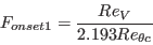


![F_{onset3} = max \left[ 1 - \left( \frac{R_T}{2.5} \right)^3, 0 \right]](./Transitional_SSGLRR_Reynolds_Stress_Model_files/img11.png)
![F_{turb} = exp \left[ - \left( \frac{R_T}{4} \right) ^4 \right]](./Transitional_SSGLRR_Reynolds_Stress_Model_files/img12.png)

![{{F}_{sublayer}}=exp\left[ -{{\left( \frac{R{{e}_{\lambda }}}{200} \right)}^{2}} \right]](./Transitional_SSGLRR_Reynolds_Stress_Model_files/img15.png)

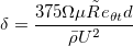
![Re_{\theta c}=f_{\theta c}\tilde{R}e_{\theta t},
f_{\theta c}=0.99-0.37\Big\{1-\exp\Big[-\max\Big(0,\frac{\tilde{R}e_{\theta t}+40}{320}\Big)\Big]\Big\}^2](./Transitional_SSGLRR_Reynolds_Stress_Model_files/Rethetac.png)
The source term of the  equation is defined as:


![F_{\theta t} = min \left[ max \left( F_{wake} exp \left(- \left( \frac{d}{\delta} \right) ^4 \right) , 1.0 - \left( \frac{c_{e2}\gamma - 1}{c_{e2} - 1}\right) ^2 \right), 1.0 \right]](./Transitional_SSGLRR_Reynolds_Stress_Model_files/img28.png)
![F_{wake} = exp \left[ - \left( \frac{Re_{\omega}}{1\cdot 10^{5}} \right) ^2 \right]](./Transitional_SSGLRR_Reynolds_Stress_Model_files/img30.png)

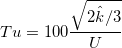
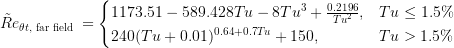
![{{\operatorname{Re}}_{\theta t}}=\left\{ \begin{array}{*{35}{l}}
\left[ 1173.51-589.428Tu-8T{{u}^{3}}+\frac{0.2196}{T{{u}^{2}}} \right]F\left( {{\lambda }_{\theta }} \right), & Tu\le %1.5 \\
\left[ 240{{(Tu+0.01)}^{0.64+0.7Tu}}+150 \right]F\left( {{\lambda }_{\theta }} \right), & Tu>%1.5 \\
\end{array} \right.](./Transitional_SSGLRR_Reynolds_Stress_Model_files/img34.png)
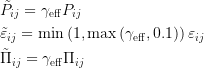
![F \left( \lambda_{\theta} \right) = \left\{
\begin{array}{ll}
1 + \left[ 12.986 \lambda_{\theta} + 123.66 \lambda_{\theta} ^2 + 405.689 \lambda_{\theta} ^3 \right] exp \left( -\left( \frac{Tu}{1.5} \right)^{1.5} \right), & \lambda_{\theta} \leq 0; \\
1 + 0.275 \left[1 - exp \left( -35.0 \lambda_{\theta} \right) \right] exp \left( - \frac{Tu}{0.5} \right) & \lambda_{\theta} > 0
\end{array} \right.](./Transitional_SSGLRR_Reynolds_Stress_Model_files/img35.png)
IMPORTANT: The expression for  is an implicit function of
  through the presence of
  since
since
 are typically
solved by iterating on the value of ).
Note that in the nomenclature of AIAA Journal 47(12):2894-2906, 2009, the expression for
uses a "local freestream velocity" for U, which is actually
intended to be the velocity at the edge of the boundary layer. But in the functionality
of the model, this velocity needs to be the local velocity. Although
is small for small velocities (i.e. near the wall
in a boundary layer), this effect is accounted for in the model with the F_theta_t term. Outside of the boundary layer, the transported
is "attracted" to the equilibrium value
() and is physically correct at the edge of the boundary layer.
Inside the boundary layer, the attraction is suppressed and the value at the edge is diffused into the boundary layer.
are typically
solved by iterating on the value of ).
Note that in the nomenclature of AIAA Journal 47(12):2894-2906, 2009, the expression for
uses a "local freestream velocity" for U, which is actually
intended to be the velocity at the edge of the boundary layer. But in the functionality
of the model, this velocity needs to be the local velocity. Although
is small for small velocities (i.e. near the wall
in a boundary layer), this effect is accounted for in the model with the F_theta_t term. Outside of the boundary layer, the transported
is "attracted" to the equilibrium value
() and is physically correct at the edge of the boundary layer.
Inside the boundary layer, the attraction is suppressed and the value at the edge is diffused into the boundary layer.
The calibration constants for the Langtry-Menter model are:
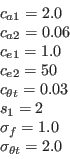 and are:


The effects of laminar-turbulent transition are introduced to the underlying SSG/LRR model by modifying the source terms as:
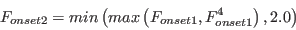
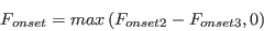
For numerical robustness, the following three limits are enforced:


This model is not Galilean invariant, due to its explicit use of the velocity vector.
Return to: Turbulence Modeling Resource Home Page
Shengye Wang is acknowledged for helping with this webpage.
Recent significant updates:
Responsible NASA Official:
Christopher Rumsey
Page Curator:
Christopher Rumsey
Last Updated: 04/08/2025