
 |
Langley Research CenterTurbulence Modeling Resource |
The SA-noft2-Gamma-Retheta 3-equation Transitional Model
This web page gives detailed information
on the equations for various forms of the
SA-noft2-Gamma-Retheta transition modeling framework.
All forms of the model given on this page are linear eddy viscosity models.
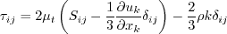
Linear models use the Boussinesq assumption for the constitutive relation:
Unless otherwise stated, for compressible flow with heat transfer this model is implemented as described on the page
Implementing Turbulence Models into the Compressible RANS Equations, with perfect gas
assumed and Pr = 0.72, Prt = 0.90, and Sutherland's law for dynamic viscosity.
Return to: Turbulence Modeling Resource Home Page SA-noft2-Gamma-Retheta 3-equation Transition Model
(SA-noft2-Gamma-Retheta)
This model is result of the coupling of the Spalart-Allmaras (SA-noft2) model with the Langtry-Menter
local correlation based transition approach.
The SA-noft2 model is augmented by two additional equations, originally developed by
Menter et al. (Flow Turb Combust 77:277-303, 2006) in the the k-omega equations context, for transitional flows.
The primary references for the implementation of this model are:
Like the SST-2003-LM2009 model on which it is partially based,
this model is not Galilean invariant, due to its explicit use of the velocity vector.
The transport equations to take into account transition are given by following:
The source terms in the
The main transport equation from SA-noft2 is modified in the following way, in order to take into account the transitional effects:
where
with
The following closure constants are also adopted for the SA-noft2 equation:
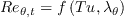
Model Empirical Correlations
The present model contains, as other
where Tu is the turbulence intensity and
In the literature, a strong sensitivity of gamma-Retheta models to the
Boundary Conditions
Standard boundary conditions are adopted for
It also is very important to remark that in order to capture the
laminar and transitional boundary layers
correctly, the grid must have a first cell height, viscous sublayer scaled, y+
of no more than approximately 1.
SA-noft2-LRe-Gamma-Retheta 3-equation Transition Model
(SA-noft2-LRe-Gamma-Retheta)
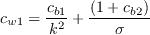
This model is the same as (SA-noft2-Gamma-Retheta)
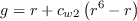
except that the low Reynolds number correction is included by modifying cw2 (see
SA-LRe).
Return to: Turbulence Modeling Resource Home Page Andrea Zoppi and Valerio D'Alessandro of Università Politecnica delle Marche (Italy) are
acknowledged for helping put together this webpage.
Recent significant updates: Responsible NASA Official:
Ethan Vogel
![\frac{\partial (\rho\gamma)}{\partial t} + \frac{\partial (\rho u_j \gamma)}{\partial x_j} = \rho P_\gamma - \rho D_\gamma +
\frac{\partial}{\partial x_j}\left[
\left( \mu + \frac{\mu_t}{\sigma_f}\right) \frac{\partial \gamma}{\partial x_j} \right]](SAnoft2_gamma_retheta_eqns/img75.png)
(In the original references, these equations were written in incompressible form, as follows:
![\frac{\partial (\rho \widehat{Re}_{\theta,t})}{\partial t} + \frac{\partial (\rho u_j \widehat{Re}_{\theta,t}) }{\partial x_j} =
\rho P_{\theta,t} + \frac{\partial}{\partial x_j} \left[
\sigma_{\theta,t} \left( \mu + \mu_t \right) \frac{\partial \widehat{Re}_{\theta,t}}{\partial x_j} \right]](SAnoft2_gamma_retheta_eqns/img76.png)
![\frac{\partial \gamma}{\partial t} + u_j \frac{\partial \gamma}{\partial x_j} = P_\gamma - D_\gamma + \frac{\partial}{\partial x_j}\left[
\left( \nu + \frac{\nu_t}{\sigma_f}\right) \frac{\partial \gamma}{\partial x_j} \right]](SAnoft2_gamma_retheta_eqns/img2.png)
![\frac{\partial \widehat{Re}_{\theta,t}}{\partial t} + u_j \frac{\partial \widehat{Re}_{\theta,t} }{\partial x_j} = P_{\theta,t} + \frac{\partial}{\partial x_j} \left[
\sigma_{\theta,t} \left( \nu + \nu_t \right) \frac{\partial \widehat{Re}_{\theta,t}}{\partial x_j} \right]](SAnoft2_gamma_retheta_eqns/img3.png)
 equation are defined as:
![P_\gamma = c_{a1} S \left[ \gamma F_{onset} \right]^{0.5} \left(1 - c_{e1} \gamma \right) F_{length}](SAnoft2_gamma_retheta_eqns/img5.png)
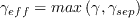
In 
 , the term
 is computed as:
with


![F_{onset,3} = max \left[\left( 2 - \left( \frac{R_T}{2.5} \right)^3 \right), 0 \right]](SAnoft2_gamma_retheta_eqns/img11.png)
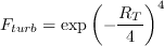
The terms 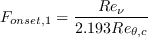
 and
and
 are obtained as follows:
 and
and
 .
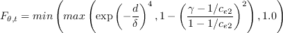
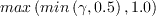
On the other hand, for the destruction term,
.
On the other hand, for the destruction term,
 , the coefficient
 is defined:
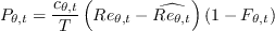
As regards the source terms in the transport equation for
 ,
the following equation is adopted:
,
the following equation is adopted:
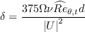
The last term is defined as:
where
Additionally, the term T appearing in the source term of the
 equation is defined as follows:
The following closure constants are adopted in order to close the transport equations for transition:

 ,
,
 ,
,
 ,
,
 ,
,
 ,
,
 ,
,
 .
.
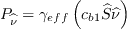
where
![\frac{\partial \widehat \nu}{\partial t} + u_j \frac{\partial \widehat \nu}{\partial x_j} =
P_{\widehat \nu} - D_{\widehat \nu} +
\frac{1}{\sigma} \left[ \frac{\partial}{\partial x_j}
\left( \left( \nu + \widehat \nu \right) \frac{\partial \widehat \nu}{\partial x_j} \right)
+ {c_{b2}}\frac{\partial \widehat \nu}{\partial x_i} \frac{\partial \widehat \nu}{\partial x_i}
\right]](SAnoft2_gamma_retheta_eqns/img33.png)
(Note: earlier versions had a 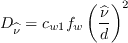
 multiplying this term, but this was a holdover from
previous code modifications, and is simply unity all the time.)
multiplying this term, but this was a holdover from
previous code modifications, and is simply unity all the time.)
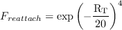
and
![\gamma_{sep} = min \left( 2.0 \cdot max \left[ 0 , \left( \frac{Re_\nu}{3.235 Re_{\theta,c}} \right) -1\right]
F_{reattach}, 2.0 \right)F_{\theta,t}](SAnoft2_gamma_retheta_eqns/img37.png)
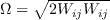
The following closure functions complete the definition of the SA-noft2 equation:
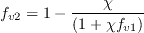
![f_{w} = g\left[ \frac{1+c_{w3}^6}{g^6 + c_{w3}^6} \right]^{\frac{1}{6}}](SAnoft2_gamma_retheta_eqns/img42.png)
![\widehat S = \left[\Omega + min\left( 0 , S-\Omega \right)\right] + \frac{\widehat{\nu}}{k^2d^2}f_{v2}](SAnoft2_gamma_retheta_eqns/img43.png)
where 
 is the dimensionless turbulent variable,
 is the vorticity tensor module, and
 .
.
 ,
,
 ,
,
 ,
,
 ,
,
 ,
,
 ,
,
 , and
, and
 .
.
 approaches available in literature,
three empirical correlations needed to compute
approaches available in literature,
three empirical correlations needed to compute
 ,
,
 , and
, and
 .
In the seminal contribution of Menter et al. (Flow Turb Combust 77:277-303, 2006), these three variables
are related to:
.
In the seminal contribution of Menter et al. (Flow Turb Combust 77:277-303, 2006), these three variables
are related to:
 ,
,
 , and
, and
 ,
,
 is the Thwaites' pressure gradient coefficient:
These correlations were not released immmediately
since they were proprietary.
For this reason a specific literature segment
containing several approaches for these correlations was started.
In D'Alessandro et al. (Energy 130:402-419, 2017) and Zoppi (PhD Thesis), various approaches, developed within SST k-omega, were tested
and compared for the current model.
The best performance in terms of
 were found using an expression developed by Menter et al.:
where

It is important to remark that in the above correlations
![F\left(\lambda_\theta \right) = \left\{ \begin{array}{l}
1 + \left[12.986 \lambda_\theta + 123.66 \lambda_\theta^2 + 405.689 \lambda_\theta^3 \right] \exp\left( - \left( \frac{Tu}{1.5} \right)^{1.5}\right) ...{for}... \lambda_\theta \leq 0\\
1+ 0.275\left[1-\exp\left( -35 \lambda_\theta \right)\right] \exp\left( -\frac{Tu}{0.5} \right) ...{for}... \lambda_\theta >0
\end{array}](SAnoft2_gamma_retheta_eqns/img66.png)
 is used for all the points of the flowfield.
Moreover,
is computed by
iterating on the value of
is used for all the points of the flowfield.
Moreover,
is computed by
iterating on the value of
 ,
since
is a function of
itself through the presence of
,
since
is a function of
itself through the presence of
 .
and
correlations (as well as transition
criteria used to compute
)
has been documented.
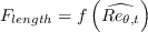
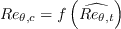
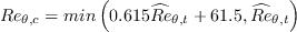
There are many different correlations for
and
to choose from
(see Tables 1 and 2 in D'Alessandro et al., Energy, 130:402-419, 2017).
However, it was noted in that reference
that the Malan et al. correlation (Malan et al. AIAA-2009-1142, 2009,
https://doi.org/10.2514/6.2009-1142) provides the best performance for the
flowfields developing around low-Reynolds number operating airfoils. These correlations are:
.
and
correlations (as well as transition
criteria used to compute
)
has been documented.
There are many different correlations for
and
to choose from
(see Tables 1 and 2 in D'Alessandro et al., Energy, 130:402-419, 2017).
However, it was noted in that reference
that the Malan et al. correlation (Malan et al. AIAA-2009-1142, 2009,
https://doi.org/10.2514/6.2009-1142) provides the best performance for the
flowfields developing around low-Reynolds number operating airfoils. These correlations are:

 ,
the Spalart-Allmaras variable:
,
the Spalart-Allmaras variable:
 in the freestream and
 .
The boundary condition for
at the wall is zero normal flux.
At an inlet or freestream, the value of
is equal to 1.
The boundary condition for
at the wall is
zero flux, while at an inlet or freestream
is calculated from the specific empirical
correlation based on the inlet turbulence intensity.
.
The boundary condition for
at the wall is zero normal flux.
At an inlet or freestream, the value of
is equal to 1.
The boundary condition for
at the wall is
zero flux, while at an inlet or freestream
is calculated from the specific empirical
correlation based on the inlet turbulence intensity.
02/06/2023 - clarified the form of the destruction term in the SA equation
Page Curator:
Clark Pederson
Last Updated: 02/06/2023