Results are shown here from 2 compressible codes
so that the user may compare their own compressible code results. Multiple grids were
used so the user can see trends with grid refinement. Different codes will behave
differently with grid refinement depending on many factors (including code order of accuracy
and other numerics),
but it would be expected that as the grid is refined the results
will tend toward an "infinite grid" solution that is the same.
Be careful when comparing details: any differences in boundary conditions or flow conditions
may affect results.
Two independent compressible RANS codes,
CFL3D and FUN3D, were used to compute this
bump-in-channel flow with the Spalart-Allmaras turbulence model with Rotation-Curvature correction
(version SA-RC - see full description on
Spalart-Allmaras page). Compare results here with those on the
SA Expected Results - 2D Bump-in-channel page to see the effect of the
Rotation-Curvature terms for this case. The full series of 5 grids were used.
CFL3D is a cell-centered structured-grid code, and FUN3D
is a node-centered unstructured-grid code (FUN3D can solve on mixed element grids, so this case
was computed on the same hexahedral grid used by CFL3D). Both codes used Roe's Flux Difference
Splitting and a UMUSCL upwind approach. In CFL3D its standard UMUSCL (kappa=0.33333) scheme was
used, whereas in FUN3D the option UMUSCL 0.5 was used. Both codes were run with
full Navier-Stokes (as opposed to thin-layer, which is CFL3D's default mode of operation),
and both codes used first-order upwinding for the advective terms of the turbulence model.
Details about the codes can be found on their respective websites,
the links for which are given on this site's
home page.
The codes were not run to machine-zero iterative convergence, but an attempt was made to converge
sufficiently so that results of interest were well within normal engineering tolerance and
plotting accuracy. For example, for CFL3D the density residual was typically
driven down below 10-13. It should be kept in mind that many of the files given below
contain computed values directly from the codes,
using a precision greater than the convergence tolerance (i.e., the values
in the files are not necessarily as precise as the number of digits given).
For the CFL3D and FUN3D tests reported below, the turbulent inflow boundary condition used for SA was:
 .
In both CFL3D and FUN3D, this was not the default setting, so special keywords needed to be
set in both codes.
For the interested reader, typical input files for this problem are given here:
CFL3D V6.5:
FUN3D:
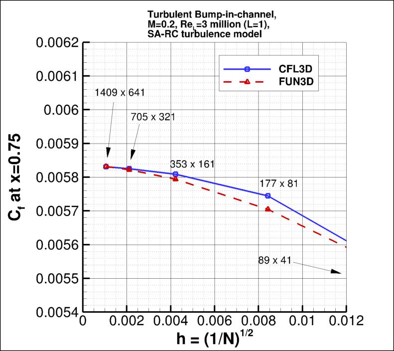
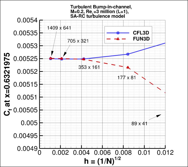
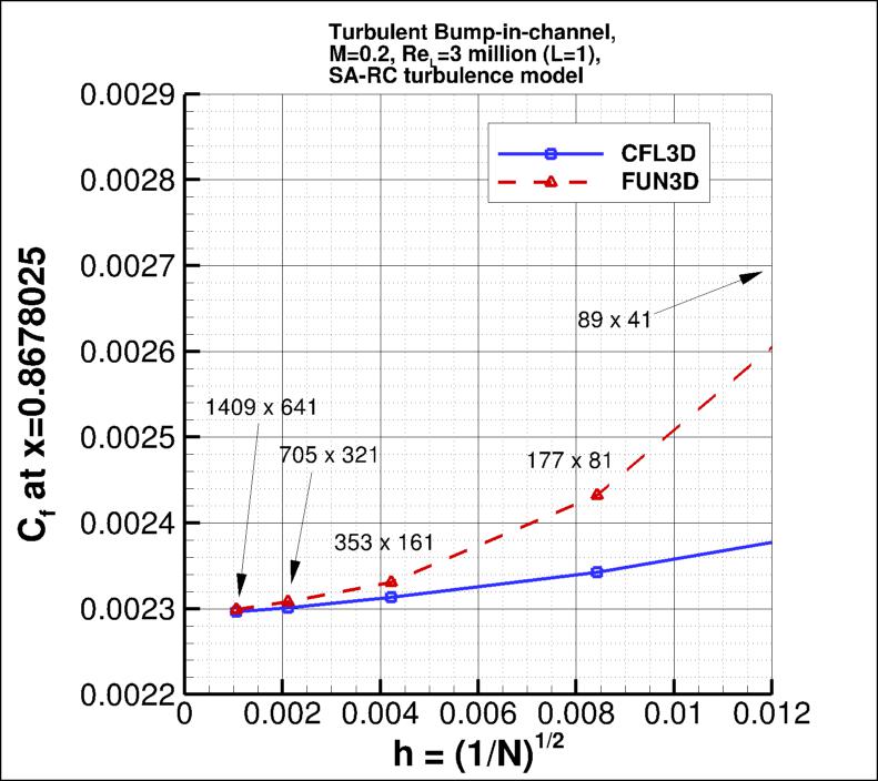
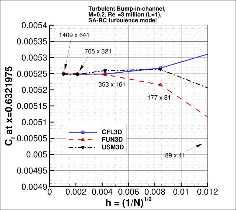
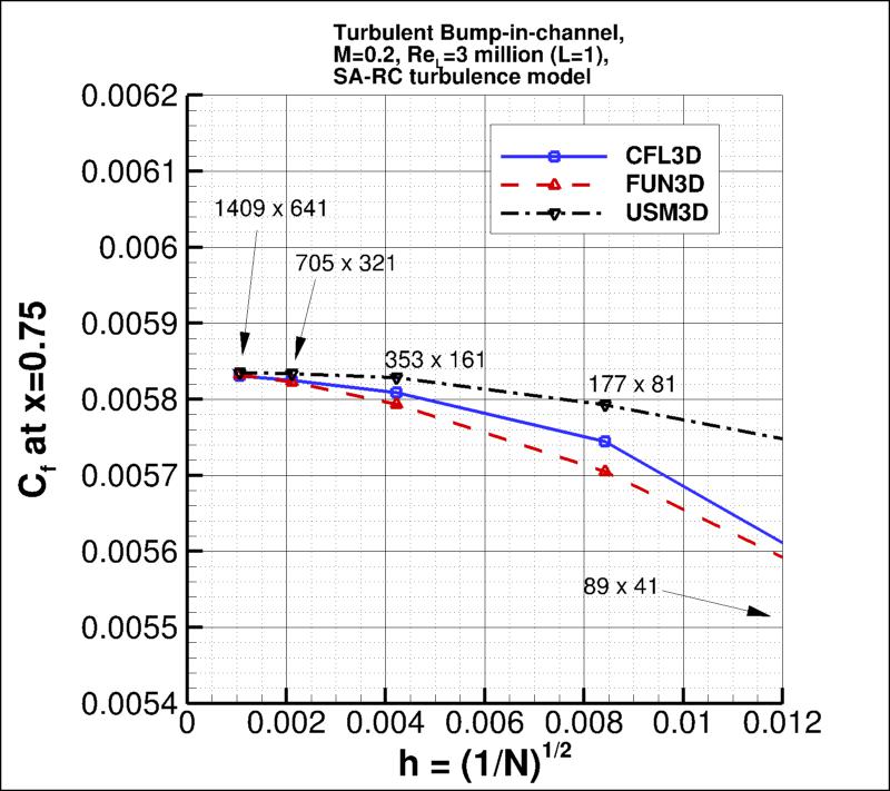
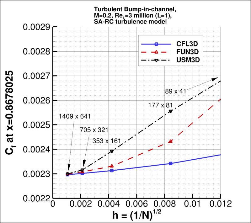
The following plots show the convergence of the wall skin friction coefficient
at the bump peak (at x=0.75), in front of the bump peak (at x=0.6321975), and
aft of the peak (at x=0.8678025) with
grid size for the two codes.
In the plot the x-axis is plotting 1/N1/2, which is proportional to
grid spacing (h).
At the left of the plot, h=0 represents an infinitely fine grid.
Both codes go toward approximately the same result on an infinitely refined grid.
Using the uncertainty estimation procedure from the Fluids Engineering Division of the ASME (Celik, I. B.,
Ghia, U., Roache, P. J., Freitas, C. J., Coleman, H., Raad, P. E.,
"Procedure for Estimation and Reporting of Uncertainty Due
to Discretization in CFD Applications," Journal of Fluids Engineering, Vol. 130, July 2008, 078001, https://doi.org/10.1115/1.2960953), described in Summary of Uncertainty Procedure,
the finest 3 grids yield the following for skin friction coefficient at x=0.75, x=0.6321975, and
x=0.8678025:
| Code |
Computed apparent order, p |
Approx rel fine-grid error, ea21 |
Extrap rel fine-grid error, eext21 |
Fine-grid convergence index, GCIfine21 |
| x=0.75 |
| CFL3D |
1.50 |
0.099% |
0.054% |
0.068% |
| FUN3D |
1.57 |
0.165% |
0.084% |
0.105% |
| x=0.6321975 |
| CFL3D |
oscillatory convergence |
0.021% |
N/A |
N/A |
| FUN3D |
2.54 |
0.010% |
0.002% |
0.003% |
| x=0.8678025 |
| CFL3D |
1.34 |
0.200% |
0.130% |
0.163% |
| FUN3D |
1.43 |
0.375% |
0.222% |
0.277% |
The data file that generated the above plot is given here:
cf_convergence_sarc.dat.
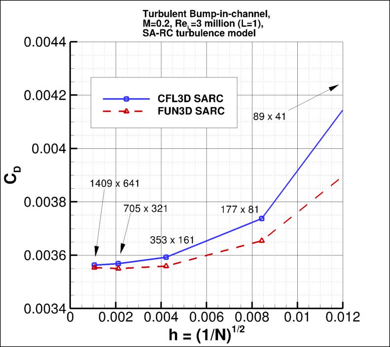
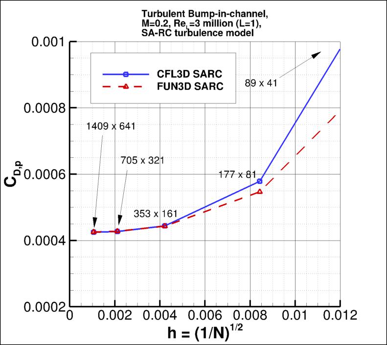
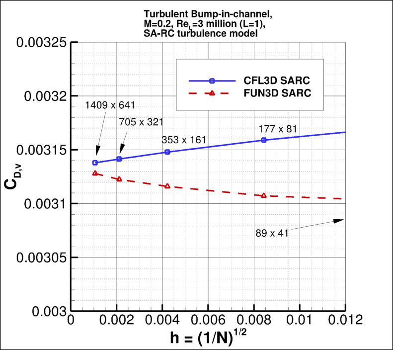
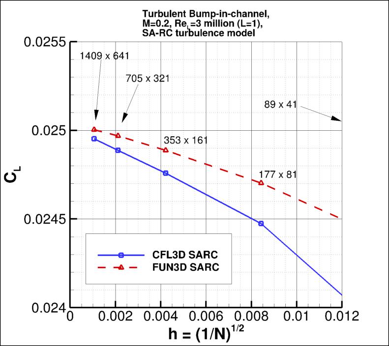
The following plots show: (1) total drag coefficient, (2) pressure drag coefficient,
(3) viscous drag coefficient, and (4) total lift coefficient for the bump.
In this bump case the surface skin friction
is singular (tends toward infinity) at the leading edge. The finer the grid, the more nearly singular
the local behavior on a finite grid.
There is also locally anomalous behavior in Cf at the back end of the bump wall (at x=1.5), as
is often seen in CFD solutions near trailing edges (see, e.g., Swanson and Turkel, AIAA Paper 87-1107, 1987
https://doi.org/10.2514/6.1987-1107).
Both of these behaviors may have some influence
on the convergence/order-property of the integrated viscous component of the drag coefficient.
As seen in the following plots, both codes are tending toward similar integrated force coefficient values
as the grid is refined.


Using the uncertainty estimation procedure from the Fluids Engineering Division of the ASME (Celik, I. B.,
Ghia, U., Roache, P. J., Freitas, C. J., Coleman, H., Raad, P. E.,
"Procedure for Estimation and Reporting of Uncertainty Due
to Discretization in CFD Applications," Journal of Fluids Engineering, Vol. 130, July 2008, 078001, https://doi.org/10.1115/1.2960953), described in Summary of Uncertainty Procedure,
the finest 3 grids yield the following for force coefficients:
| Code |
Quantity |
Computed apparent order, p |
Approx rel fine-grid error, ea21 |
Extrap rel fine-grid error, eext21 |
Fine-grid convergence index, GCIfine21 |
| CFL3D |
Cd |
2.12 |
0.151% |
0.045% |
0.057% |
| CFL3D |
Cd,p |
3.13 |
0.458% |
0.059% |
5.590% |
| CFL3D |
Cd,v |
0.88 |
0.110% |
0.131% |
0.164% |
| CFL3D |
CL |
0.99 |
0.260% |
0.264% |
0.331% |
| FUN3D |
Cd |
oscillatory convergence |
0.090% |
N/A |
N/A |
| FUN3D |
Cd,p |
2.79 |
0.524% |
0.089% |
0.111% |
| FUN3D |
Cd,v |
0.25 |
0.173% |
0.922% |
0.473% |
| FUN3D |
CL |
1.21 |
0.140% |
0.106% |
0.132% |
The data file that generated the above plot is given here:
force_convergence_sarc.dat.
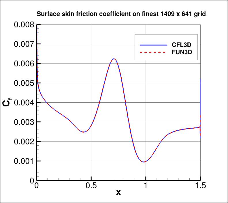
The surface skin friction coefficient from both codes on the finest 1409 x 641 grid
over the entire bump wall is shown in the next plot. Again, local anomalous behavior exists near the leading
edge (x=0) due to singular behavior of the solution,
as well as near the trailing edge (x=1.5) due to numerical influences.
These behaviors differ for the two codes, and result in small local deviations that
can be seen when zoomed into the two locations. But both codes are seen to yield nearly identical results
over most of the bump wall.
The data file that generated the above plot is given here:
cf_bump_sarc.dat.
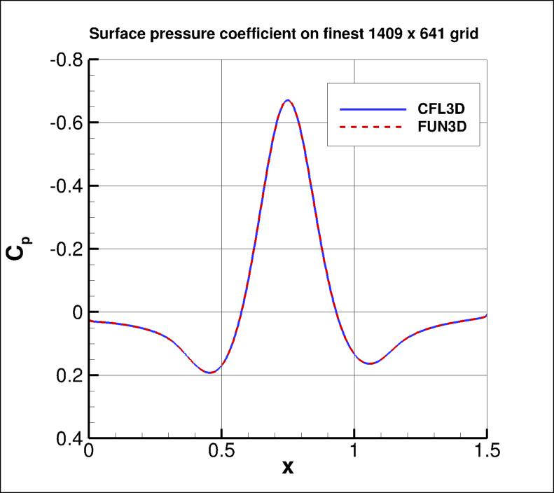
The surface pressure coefficient from both codes on the finest 1409 x 641 grid
over the entire bump wall is shown in the next plot.
Both codes yield nearly identical results.
The data file that generated the above plot is given here:
cp_bump_sarc.dat.
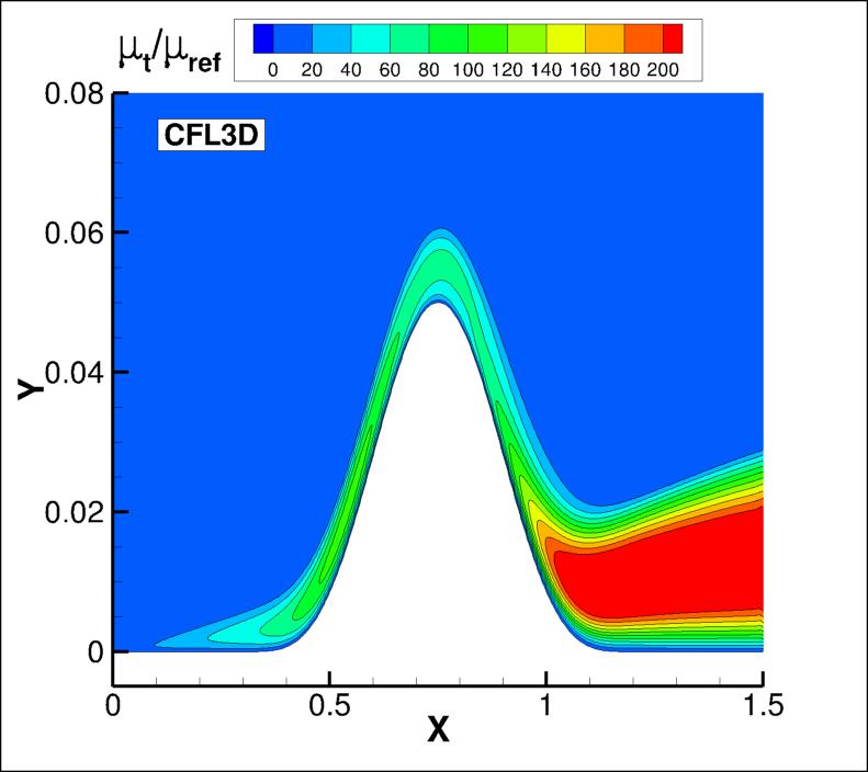
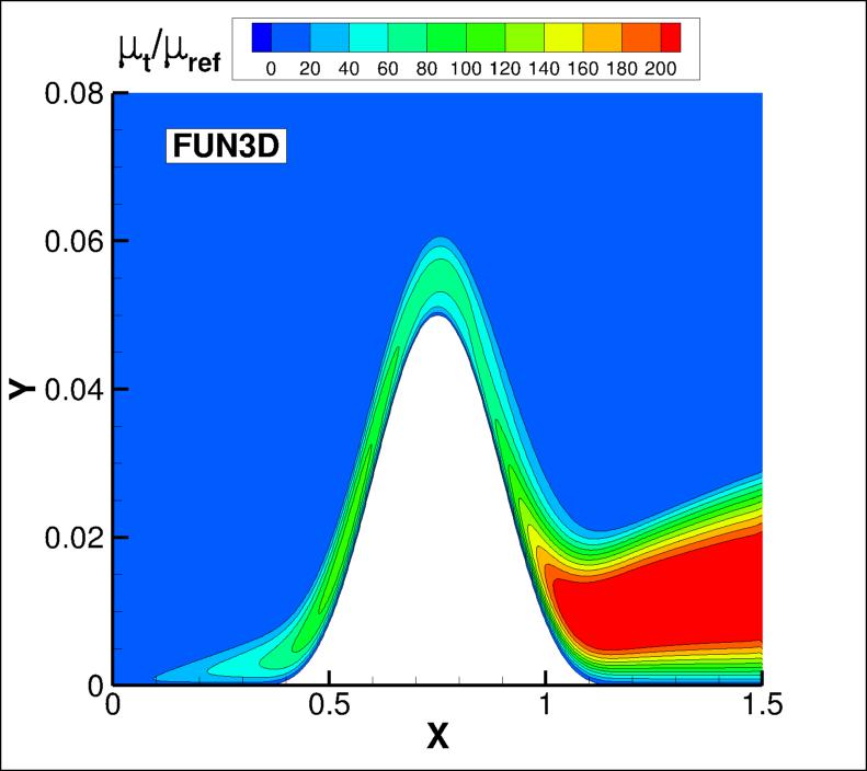
The eddy viscosity contours (nondimensionalized by freestream laminar viscosity)
from the two codes on the finest 1409 x 641 grid are shown
in the following plots (y-scale expanded for clarity). They are essentially indistinguishable.
(Note legends do not necessarily reflect min and max values.)
The data files that generated the above plots are given here:
mut_contours_cfl3d_sarc.dat.gz (9.7 MB) (structured, at cell centers) and
mut_contours_fun3d_sarc.dat.gz (16.7 MB) (unstructured, at grid points). Note
that these are both gzipped
Tecplot
formatted files, so you must either have Tecplot or know how to read their format in order to use these
files.
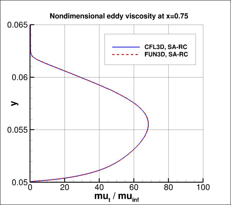
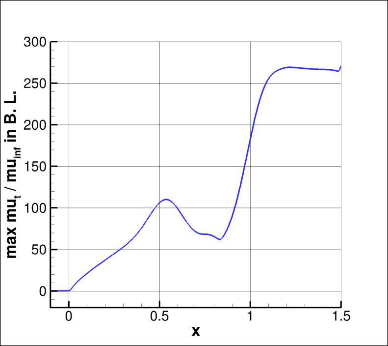
Using the finest 1409 x 641 grid, an extracted nondimensional eddy viscosity profile at
x=0.75 is shown below, along with a plot of the maximum nondimensional
eddy viscosity as a function of x.
The data file that generated the eddy viscosity profile at x=0.75 is given here:
mut_0.75_sarc.dat.
The data file that generated the max eddy viscosity plot is given here:
mut_max_sarc.dat (extracted only for CFL3D).
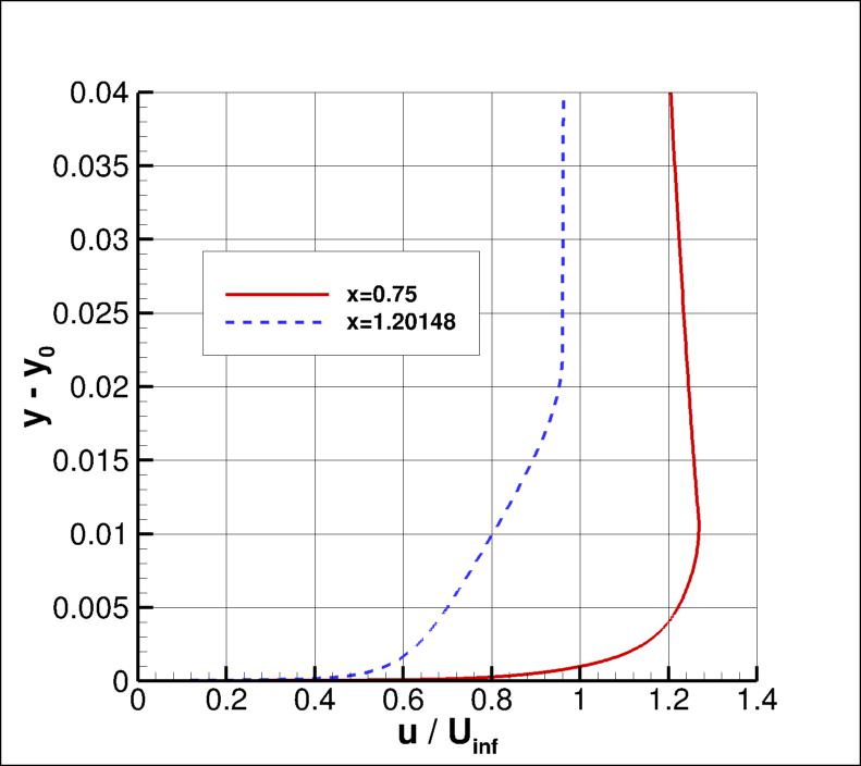
U-Velocity profiles are shown at the two x-locations of x=0.75 and x=1.20148 for
the finest grid in the following plot.
The data file that generated the above plot is given in
uvel_sarc.dat (extracted only for CFL3D).
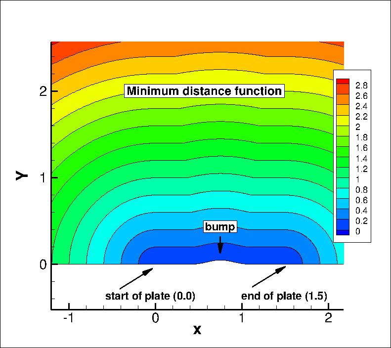
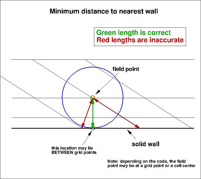
The SA model relies on the minimum distance to the nearest wall. For this case,
contours of this function
are shown in the following plot, for the grid 1 level down from the finest
grid.

The data file that generated the above plot is given in
bump_1levdown.mindist.dat.gz (gzipped file,
3.9 MB, unstructured, at grid points). Note
that this is a gzipped Tecplot
formatted file, so you must either have Tecplot or know how to read their format in
order to use it.
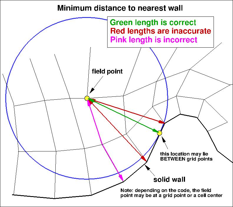
It is important to note that computing minimum distance by searching along grid lines is
incorrect, and is not the same as computing actual minimum distance to the nearest wall for this grid. Using
the former method will yield some minor differences in the results. The following sketches
demonstrate the concept of minimum distance. Improperly-calculated minimum distance
functions will particularly produce incorrect results for cases in which the
grid lines are not perfectly normal to the body surface.
Note that when the nearest wall point is a sharp convex corner or edge (like an airfoil or wing trailing edge) then the
correct minimum distance is the distance to that corner or edge, which is not a wall normal.


Results from USM3D are shown alongside the CFL3D and FUN3D results below.
All codes are converging to the same results.

 .
In both CFL3D and FUN3D, this was not the default setting, so special keywords needed to be
set in both codes.
For the interested reader, typical input files for this problem are given here:
