Return to: 3D Modified Bump-in-channel Validation for Numerical Analysis Intro Page
Return to: Turbulence Modeling Resource Home Page
TURBULENCE MODEL NUMERICAL ANALYSIS
3D Modified Bump-in-channel Validation
SA-neg Model Results
Link to SA-neg equations
Results are shown for the 3D modified bump-in-channel at M=0.2, Re=3 million based on unit length, and reference temperature
of 540 R.
Three different CFD codes (FUN3D, USM3D, and CFL3D) have been employed
in an effort to try to discern the grid-converged result for this case.
Results here
are for the SA-neg variant of the SA model.
However, SA-neg is passive to the
original (SA) model in well-resolved flowfields, and hence is expected to yield essentially identical
results as SA for the cases here.
FUN3D and USM3D both used clipping method "a" with cutoff 0.00001 for  ,
while CFL3D used clipping method "c" (see Note 1 on
the Spalart-Allmaras equation page).
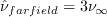
For all codes, the farfield value of the Spalart turbulence variable is
,
while CFL3D used clipping method "c" (see Note 1 on
the Spalart-Allmaras equation page).
For all codes, the farfield value of the Spalart turbulence variable is
 .
In all codes the Prandtl number Pr is taken to be constant at 0.72, and turbulent Prandtl
number Prt is taken to be constant at 0.9.
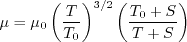
The dynamic viscosity is computed using
Sutherland's Law (See White, F. M., "Viscous Fluid Flow," McGraw Hill, New York, 1974, p. 28).
In Sutherland's Law, the local value of dynamic viscosity is determined by plugging the local value of temperature
(T) into the following formula:
.
In all codes the Prandtl number Pr is taken to be constant at 0.72, and turbulent Prandtl
number Prt is taken to be constant at 0.9.
The dynamic viscosity is computed using
Sutherland's Law (See White, F. M., "Viscous Fluid Flow," McGraw Hill, New York, 1974, p. 28).
In Sutherland's Law, the local value of dynamic viscosity is determined by plugging the local value of temperature
(T) into the following formula:
where
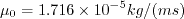 ,
,
 , and
, and
 .
The same formula can be found online
(with temperature constants given in degrees K and some small conversion differences).
Note that in terms of the reference quantities for this particular case, Sutherland's Law can equivalently be written:
.
The same formula can be found online
(with temperature constants given in degrees K and some small conversion differences).
Note that in terms of the reference quantities for this particular case, Sutherland's Law can equivalently be written:
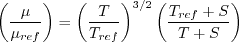
where
 is the reference dynamic viscosity that corresponds to the freestream in this case, and
freestream
is the reference dynamic viscosity that corresponds to the freestream in this case, and
freestream  (as defined on the
previous
page) is 540R. This latter form may be more convenient for nondimensional codes.
(Specific details regarding an implementation of Sutherland's Law in nondimensional codes can be found in
handwritten notes describing Sutherland's Law in CFL3D and FUN3D.)
(as defined on the
previous
page) is 540R. This latter form may be more convenient for nondimensional codes.
(Specific details regarding an implementation of Sutherland's Law in nondimensional codes can be found in
handwritten notes describing Sutherland's Law in CFL3D and FUN3D.)
For this flow, an odd-even decoupling was originally observed in FUN3D on finer grids using the unweighted least-square
gradient. This decoupling was particularly noticeable, for example, in plots of Cp along a spanwise grid line
somewhat upstream of the bump peak.
Preliminary studies indicate the decoupling is associated with gradients near the inflection point
in the bump surface.
The decoupling was eliminated in FUN3D
by using a mapping method based on distance from the surface for
the mean flow inviscid fluxes. See AIAA paper 2016-0858,
https://doi.org/10.2514/6.2016-0858.
Note that FUN3D and USM3D both ran this
case with first order spatial accuracy on the turbulence advection term, whereas CFL3D used second order.
Grid Convergence Behavior of Forces and Maximum Eddy Viscosity
Plots are shown to illustrate grid convergence for the lift and drag coefficients.
The contributions to the drag coefficient due to the viscosity and pressure are presented separately.
Recall that all codes were run using SA-neg.
Results that generated the above plots can be found in the following data files:
fun3d_liftdrag_convergence_sa.dat,
usm3d_liftdrag_convergence_sa.dat,
cfl3d_liftdrag_convergence_sa.dat.
The plot below shows grid convergence of the maximum nondimensional eddy viscosity in the field.

Results that generated the above plot can be found in the following data files:
fun3d_mut_convergence_sa.dat,
usm3d_mut_convergence_sa.dat,
cfl3d_mut_convergence_sa.dat.
Cp Axially
The overall Cp distribution (axially, on the body along y=0)
from the three codes on the finest grid are shown in the following figure. All
results are indistinguishable to plotting accuracy.

Zooming in to the minimum Cp region, the effect of grid for each of the three codes is shown in the
following figures:
Results that generated the above plots can be found in the following data files:
fun3d_cp_axial_sa.dat,
usm3d_cp_axial_sa.dat,
cfl3d_cp_axial_sa.dat.
Cp Along a Spanwise Grid Line
The following plots show Cp along a line on the surface of the bump, defined along:
x=0.690420848175 + 0.3*(sin(pi*y))**4
The effect of grid for each code is shown. Grid 4 is too coarse, and yields very poor results.
Results that generated the above plots can be found in the following data files:
fun3d_cp_spanwise_sa.dat,
usm3d_cp_spanwise_sa.dat,
cfl3d_cp_spanwise_sa.dat.
Flowfield Along a Vertical Line Behind the Bump
The following plots show a variety of flowfield quantities along a vertical line located at x=1.207912207,
y=-0.125.
First, Cp is plotted. Then, the following
nondimensional variables are shown: u/a_ref, v/a_ref, w/a_ref, and mu_t/mu_ref.
Results that generated the above plots can be found in the following data files:
fun3d_flow_vert_sa.dat,
usm3d_flow_vert_sa.dat,
cfl3d_flow_vert_sa.dat.
Results that generated the above plots can be found in the following data files:
fun3d_mut_vert_sa.dat,
usm3d_mut_vert_sa.dat,
cfl3d_mut_vert_sa.dat.
Recall that the order of accuracy of the turbulent advection is 1st order for FUN3D and USM3D, and 2nd order
for CFL3D in all the results shown so far.
This order of accuracy has some minor noticeable influence
on the eddy viscosity in the solution, as can be demonstrated by running CFL3D with 1st order turbulence advection and comparing results.
Overall, the maximum eddy viscosity in the field is affected somewhat on any given grid, although it still
appears to be approaching the same value on an infinite grid (see first plot below).
The effect on a specific eddy viscosity profile located at x=1.207912207, y=-0.125 is demonstrated in the second plot below.
As can be seen, on the finest grid the results from the three codes
are almost identical when the same order of accuracy is employed.
The effect of higher accuracy is to yield slightly larger maximum eddy viscosity, as well as to "sharpen"
the edge of the profile near z = 0.022 - 0.024.
The third plot shows detail near the edge of turbulence, including the progression with grid refinement
on the three finest grids. It appears (for both 1st and 2nd order turbulence advection) that grid refinement drives toward a
"sharper" edge, but use of 2nd order turbulence advection approaches there faster (i.e., sharper result with less grid points).
The fourth plot shows detail near the peak eddy viscosity region, including the progression with grid refinement
on the three finest grids. Results using 1st order turbulence advection are still changing between grid levels, whereas
for 2nd order turbulence advection, the peak results are essentially the same on the 2 finest grids.
")


CFL3D results with 1st order turbulence advection can be found in the following data file:
cfl3d_mut_vert_sa_1storderturbadvect.dat.
Return to: 3D Modified Bump-in-channel Validation for Numerical Analysis Intro Page
Return to: Turbulence Modeling Resource Home Page
Recent significant updates:
11/10/2015 - sorted the FUN3D and USM3D data files
Privacy Act Statement
Accessibility Statement
Responsible NASA Official:
Ethan Vogel
Page Curator:
Clark Pederson
Last Updated: 11/08/2021


