Langley Research Center

Turbulence Modeling Resource

Return to: 3D Bump-in-channel Verification Case Intro Page

Return to: Turbulence Modeling Resource Home Page

SA Expected Results - 3D Bump-in-channel

Results are shown here from 2 compressible codes so that the user may compare their own compressible code results. Multiple grids were used so the user can see trends with grid refinement. Different codes will behave differently with grid refinement depending on many factors (including code order of accuracy and other numerics), but it would be expected that as the grid is refined the results will tend toward an "infinite grid" solution that is the same. Be careful when comparing details: any differences in boundary conditions or flow conditions may affect results.

Two independent compressible RANS codes, CFL3D and FUN3D, were used to compute this 3D bump-in-channel flow with the Spalart-Allmaras turbulence model (version SA - see full description on Spalart-Allmaras page). The full series of 5 grids were used. CFL3D is a cell-centered structured-grid code, and FUN3D is a node-centered unstructured-grid code (FUN3D can solve on mixed element grids, so this case was computed on the same hexahedral grid used by CFL3D). Both codes used Roe's Flux Difference Splitting and a UMUSCL upwind approach. In CFL3D its standard UMUSCL (kappa=0.33333) scheme was used, whereas in FUN3D the 3-D mixed-element default UMUSCL 0.5 was used. Both codes were run with full Navier-Stokes (as opposed to thin-layer, which is CFL3D's default mode of operation), and both codes used first-order upwinding for the advective terms of the turbulence model. Details about the codes can be found on their respective websites, the links for which are given on this site's home page. The codes were not run to machine-zero iterative convergence, but an attempt was made to converge sufficiently so that results of interest were well within normal engineering tolerance and plotting accuracy. For example, for CFL3D the density residual was typically driven down below 10^-12. It should be kept in mind that many of the files given below contain computed values directly from the codes, using a precision greater than the convergence tolerance (i.e., the values in the files are not necessarily as precise as the number of digits given).

For the CFL3D and FUN3D tests reported below, the turbulent inflow boundary condition used for SA was: $\tilde \nu_{farfield} \geq 3 \nu_{\infty}$ . In both CFL3D and FUN3D, this was not the default setting, so special keywords needed to be set in both codes. For the interested reader, typical input files for this problem are given here:

CFL3D V6.5:

Typical Input File for 3D Bump

FUN3D:

Note: prior to April 2, 2010, the lift and drag coefficient numbers posted on this page were scaled too high by a factor of 1.5, because an incorrect reference area (of 1 instead of 1.5) was used. This has been corrected here.

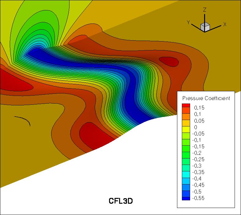
For this flow, an odd-even decoupling occurs in FUN3D on the finest grid using the default unweighted least-square gradient. This decoupling is particularly noticeable, for example, in plots of Cp along a spanwise grid line somewhat upstream of the bump peak. Preliminary studies indicate the decoupling is associated with gradients near the inflection point in the bump surface. Although not done for the results below, the decoupling can be eliminated in FUN3D by using a mapping method based on distance from the surface for the mean flow inviscid fluxes. See the 3D Modified Bump-in-channel Validation case for SA-neg in the Turbulence Model Numerical Analysis section of this website. Also see AIAA paper 2016-0858, https://doi.org/10.2514/6.2016-0858.

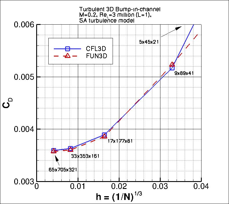
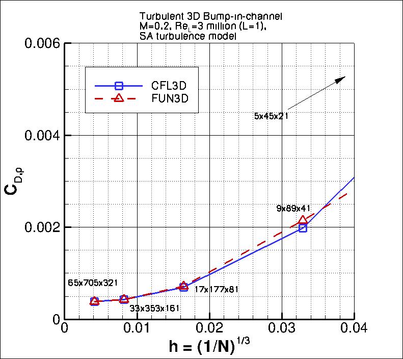
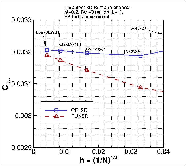
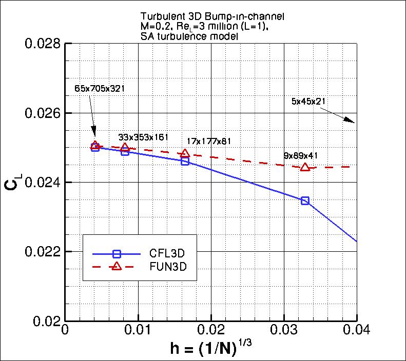
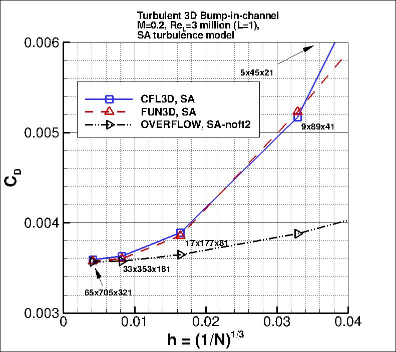
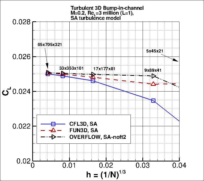
The following plots show: (1) total drag coefficient, (2) pressure drag coefficient, (3) viscous drag coefficient, and (4) total lift coefficient for the 3D bump. Both codes are tending toward similar integrated force coefficient values as the grid is refined.
convergence of 3D bump drag
coefficient vs h

convergence of 3D bump pressure drag
coefficient vs h

convergence of 3D bump viscous drag
coefficient vs h

convergence of 3D bump lift
coefficient vs h

Using the uncertainty estimation procedure from the Fluids Engineering Division of the ASME (Celik, I. B., Ghia, U., Roache, P. J., Freitas, C. J., Coleman, H., Raad, P. E., "Procedure for Estimation and Reporting of Uncertainty Due to Discretization in CFD Applications," Journal of Fluids Engineering, Vol. 130, July 2008, 078001, https://doi.org/10.1115/1.2960953), described in Summary of Uncertainty Procedure, the finest 3 grids yield the following:

Code	Quantity	Computed apparent order, p	Approx rel fine-grid error, e_a²¹	Extrap rel fine-grid error, e_ext²¹	Fine-grid convergence index, GCI_fine²¹
CFL3D	C_d	2.76	1.083%	0.188%	0.234%
CFL3D	C_d,p	2.75	10.519%	1.872%	2.297%
CFL3D	C_d,v	2.45	0.048%	0.011%	0.013%
CFL3D	C_L	1.34	0.448%	0.293%	0.367%
FUN3D	C_d	3.25	0.759%	0.089%	0.111%
FUN3D	C_d,p	2.74	11.299%	2.033%	2.491%
FUN3D	C_d,v	0.93	0.510%	0.561%	0.705%
FUN3D	C_L	1.45	0.245%	0.141%	0.177%

The data file that generated the above plots is given here: force_convergence_sa.dat.

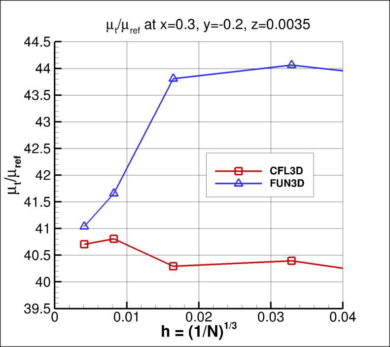
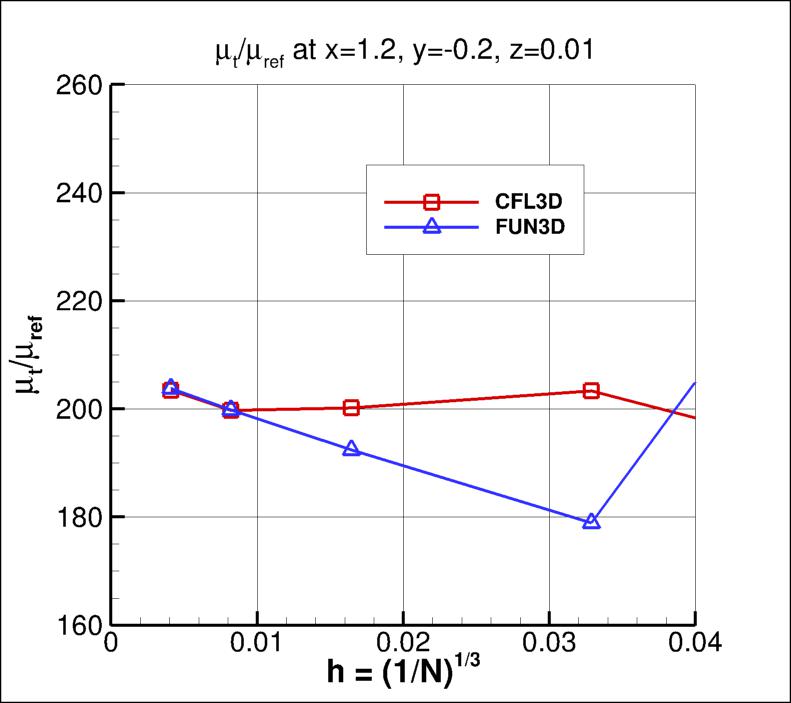
The nondimensional eddy viscosity at two particular locations in the flowfield are examined next, as a function of grid. Again, as the grid is refined (i.e., as h approaches 0), results from both codes appear to be approaching approximately the same result.
convergence of eddy viscosity at x=0.3, y=-0.2, z=0.0035 vs h

Using the same uncertainty estimation procedure as above, the finest 3 grids yield the following:

Code	Quantity	Computed apparent order, p	Approx rel fine-grid error, e_a²¹	Extrap rel fine-grid error, e_ext²¹	Fine-grid convergence index, GCI_fine²¹
CFL3D	mu_t/mu_ref at x=0.3 position	oscillatory convergence	0.254%	N/A	N/A
CFL3D	mu_t/mu_ref at x=1.2 position	oscillatory convergence	1.794%	N/A	N/A
FUN3D	mu_t/mu_ref at x=0.3 position	1.79	1.517%	0.621%	0.772%
FUN3D	mu_t/mu_ref at x=1.2 position	0.87	1.978%	2.340%	2.996%

The data file that generated the above plots is given here: eddy_convergence_sa.dat.

The surface pressure coefficient from both codes on the second-finest 33 x 353 x 161 grid over the bump wall and at y=0 is shown in the next plots. Both codes yield nearly identical results.
pressure coefficient over the bump using CFL3D

The data files that generated the above plots are given here: cp_surface_sa_cfl3d.dat.gz, cp_y0_sa_cfl3d.dat.gz, cp_surface_sa_fun3d.dat.gz, cp_y0_sa_fun3d.dat.gz. Note that these are all gzipped Tecplot formatted files, so you must either have Tecplot or know how to read their format in order to use these files.

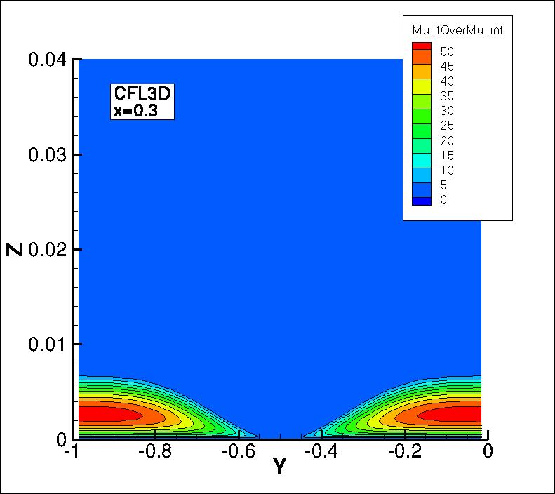
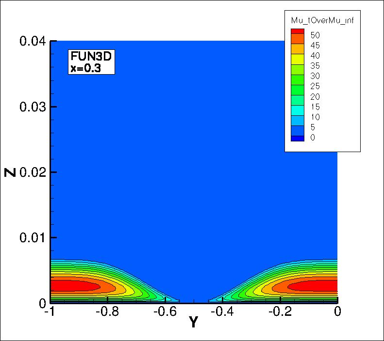
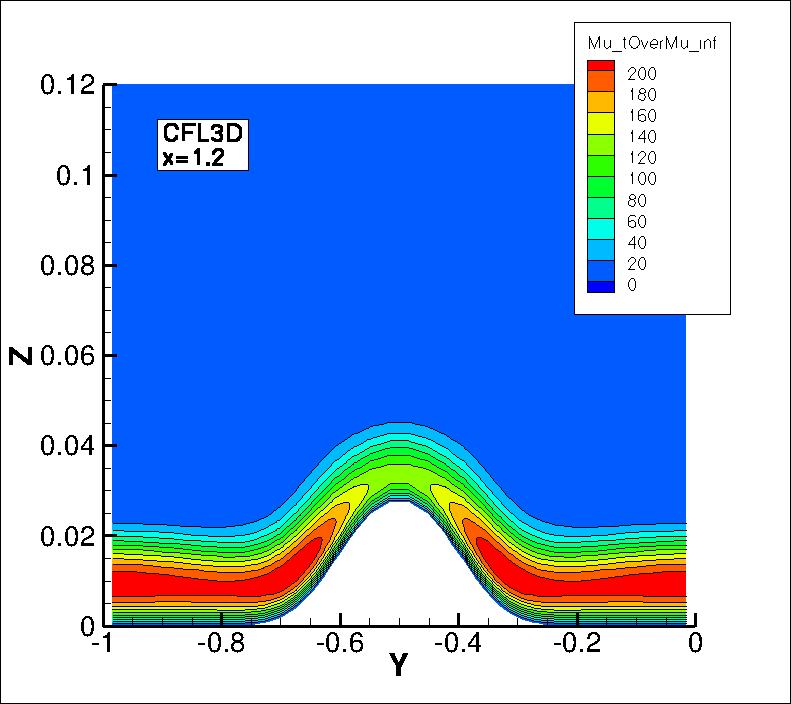
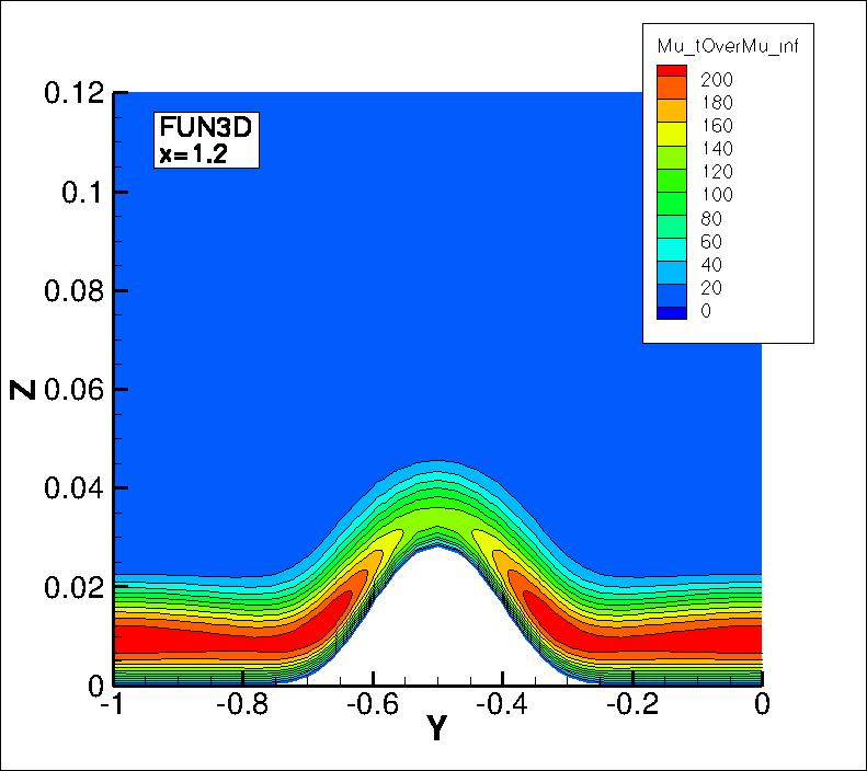
The eddy viscosity contours (nondimensionalized by freestream laminar viscosity) from the two codes on the second-finest 33 x 353 x 161 grid are shown in the following plots, extracted at two different x-locations (z-scale expanded for clarity). Results from the two codes are essentially indistinguishable. (Note legends do not necessarily reflect min and max values.)
eddy viscosity contours for CFL3D at x=0.3 eddy viscosity contours for FUN3D at x=0.3

eddy viscosity contours
for CFL3D at x=1.2 eddy viscosity contours
for FUN3D at x=1.2

The data files that generated the above plots are given here: mut_0.3_cfl3d.dat.gz, mut_0.3_fun3d.dat.gz, mut_1.2_cfl3d.dat.gz, mut_1.2_fun3d.dat.gz. Note that these are all gzipped Tecplot formatted files, so you must either have Tecplot or know how to read their format in order to use these files. Also note that the slicing tool in Tecplot was used to generate this data, extracting data along x-constant planes. These cutting planes do not necessarily coincide with grid locations. Thus, the x, y, and z locations given in the data files do not reflect actual points in the grid used.

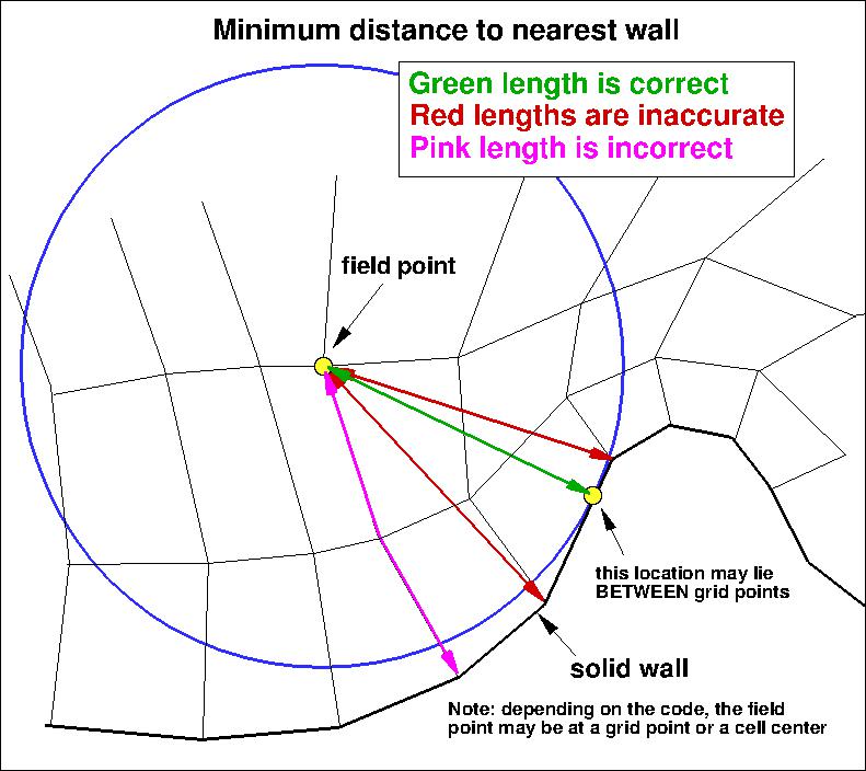
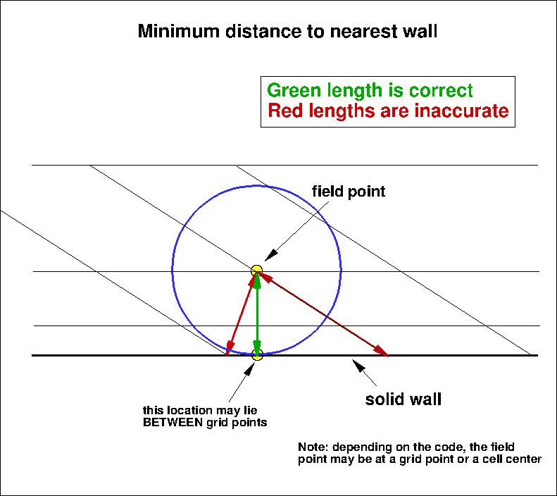
The SA model relies on the minimum distance to the nearest wall. It is important to note that computing minimum distance by searching along grid lines is incorrect, and is not the same as computing actual minimum distance to the nearest wall for this grid. The following sketches demonstrate the concept of minimum distance (in 2-D). Improperly-calculated minimum distance functions will particularly produce incorrect results for cases in which the grid lines are not perfectly normal to the body surface. Note that when the nearest wall point is a sharp convex corner or edge (like an airfoil or wing trailing edge) then the correct minimum distance is the distance to that corner or edge, which is not a wall normal.
sketch 1 demonstrating the concept of minimum distance function sketch 2 demonstrating the concept of minimum distance function

Results from OVERFLOW are shown alongside the CFL3D and FUN3D results below (note that SA-noft2 yields essentially identical results for this case as SA). NAS Technical Paper 2014-03 (pdf file) (16.2 MB) by Childs, Pulliam, and Jespersen provides details of the OVERFLOW results for this case.
convergence of 3D bump drag
coefficient vs h, incl OVERFLOW results

convergence of 3D bump lift
coefficient vs h, incl OVERFLOW results

Note for users of OpenFOAM.

Return to: 3D Bump-in-channel Verification Case Intro Page

Return to: Turbulence Modeling Resource Home Page

Recent significant updates:
02/18/2021 - added plots (and data) of eddy viscosity convergence at two paticular locations in the flowfield
07/18/2018 - added note regarding odd-even decoupling in FUN3D on finest grid for this case
12/05/2014 - added link to NAS Technical paper of OVERFLOW results for the verification cases

Privacy Act Statement

Accessibility Statement

Responsible NASA Official: Ethan Vogel
Page Curator: Clark Pederson
Last Updated: 03/01/2023