Langley Research Center

Turbulence Modeling Resource

Return to: 3D Bump-in-channel Verification Case Intro Page

Return to: Turbulence Modeling Resource Home Page

SSG/LRR-RSM-w2012 Expected Results - 3D Bump-in-channel

Results are shown here from 3 compressible codes so that the user may compare their own compressible code results. Multiple grids were used so the user can see trends with grid refinement. Different codes will behave differently with grid refinement depending on many factors (including code order of accuracy and other numerics), but it would be expected that as the grid is refined the results will tend toward an "infinite grid" solution that is the same. Be careful when comparing details: any differences in boundary conditions or flow conditions may affect results.

Three independent compressible RANS codes, CFL3D, TAU, and FUN3D, were used to compute this bump-in-channel flow with the SSG/LRR-RSM-w2012 model (see full description on SSG/LRR Full Reynolds Stress Model page). The full series of 5 grids were used. CFL3D is a cell-centered structured-grid code (NASA), TAU is a node-centered unstructured-grid code (DLR), and FUN3D is a node-centered unstructured-grid code (NASA). Both CFL3D and FUN3D used Roe's Flux Difference Splitting and a UMUSCL upwind approach. In CFL3D its standard UMUSCL (kappa=0.33333) scheme was used, whereas in FUN3D the 3-D mixed-element default UMUSCL 0.5 was used. TAU was run using central discretization with artificial matrix dissipation for the mean flow equations and upwinding for the turbulence equations. All codes were run with full Navier-Stokes (as opposed to thin-layer, which is CFL3D's default mode of operation), and all codes used first-order upwinding for the advective terms of the turbulence model. Details about the codes can be found on their respective websites (CFL3D, TAU, FUN3D). The codes were not run to machine-zero iterative convergence, but an attempt was made to converge sufficiently so that results of interest were well within normal engineering tolerance and plotting accuracy. For example, for CFL3D the density residual was typically driven down below 10^-12. It should be kept in mind that many of the files given below contain computed values directly from the codes, using a precision greater than the convergence tolerance (i.e., the values in the files are not necessarily as precise as the number of digits given).

For the CFL3D and FUN3D tests reported below, the turbulent inflow boundary conditions used for SSG/LRR-RSM-w2012 were the following:

$\hat R_{11, farfield} = \hat R_{22, farfield} = \hat R_{33, farfield} = 6 \times 10^{-9} a_{\infty}^2$

(meaning that $k_{farfield} = (\overline{u_1''u_1''} + \overline{u_2''u_2''} + \overline{u_3''u_3''})/2 = 9 \times 10^{-9} a_{\infty}^2$ ),

$\hat R_{12, farfield} = \hat R_{13, farfield} = \hat R_{23, farfield} = 0$

and

$\omega_{farfield} = 1 \times 10^{-6} \frac{\rho_{\infty}a_{\infty}^2}{\mu_{\infty}}$

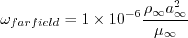
The above equations represent the "standard" SSG/LRR-RSM-w2012 boundary condition values used by CFL3D and FUN3D. In terms of freestream turbulence intensity (Tu) and freestream eddy viscosity, these boundary conditions for this particular problem (with M=0.2) correspond to: Tu=0.039% and $\mu_t / \mu = 0.009$ . The freestream values used by TAU were Tu=0.1% and $\mu_t / \mu = 0.1$ . For freestream BCs, all codes assume isotropic turbulence conditions (identical normal stresses, zero diagonal stresses).

For the interested reader, typical input files for this problem are given here:

CFL3D:

Typical Input File for 3D Bump

TAU:

Typical Input File for 3D Bump

FUN3D:

For this flow, an odd-even decoupling occurs in FUN3D on the finest grid using the default unweighted least-square gradient. This decoupling is particularly noticeable, for example, in plots of Cp along a spanwise grid line somewhat upstream of the bump peak. Preliminary studies indicate the decoupling is associated with gradients near the inflection point in the bump surface. Although not done for the results below, the decoupling can be eliminated in FUN3D by using a mapping method based on distance from the surface for the mean flow inviscid fluxes. See the 3D Modified Bump-in-channel Validation case for SA-neg in the Turbulence Model Numerical Analysis section of this website. Also see AIAA paper 2016-0858, https://doi.org/10.2514/6.2016-0858.

The following plots show: (1) total drag coefficient, (2) pressure drag coefficient, (3) viscous drag coefficient, and (4) total lift coefficient for the 3D bump. Both codes are tending toward similar integrated force coefficient values as the grid is refined.
convergence of 3D bump drag
coefficient vs h

convergence of 3D bump pressure drag
coefficient vs h

convergence of 3D bump viscous drag
coefficient vs h

convergence of 3D bump lift
coefficient vs h

Using the uncertainty estimation procedure from the Fluids Engineering Division of the ASME (Celik, I. B., Ghia, U., Roache, P. J., Freitas, C. J., Coleman, H., Raad, P. E., "Procedure for Estimation and Reporting of Uncertainty Due to Discretization in CFD Applications," Journal of Fluids Engineering, Vol. 130, July 2008, 078001, https://doi.org/10.1115/1.2960953), described in Summary of Uncertainty Procedure, the finest 3 grids yield the following:

Code	Quantity	Computed apparent order, p	Approx rel fine-grid error, e_a²¹	Extrap rel fine-grid error, e_ext²¹	Fine-grid convergence index, GCI_fine²¹
CFL3D	C_d	3.07	0.716%	0.097%	8.406%
CFL3D	C_d,p	3.08	6.142%	0.828%	72.817%
CFL3D	C_d,v	3.23	0.084%	0.010%	1.084%
CFL3D	C_L	1.28	0.567%	0.396%	0.497%
TAU	C_d	3.82	0.215%	0.016%	4.057%
TAU	C_d,p	3.01	3.958%	0.564%	0.702%
TAU	C_d,v	1.86	0.339%	0.128%	0.161%
TAU	C_L	1.42	0.119%	0.071%	0.089%
FUN3D	C_d	2.89	1.286%	0.201%	0.251%
FUN3D	C_d,p	2.92	10.774%	1.668%	2.051%
FUN3D	C_d,v	3.24	0.120%	0.014%	1.573%
FUN3D	C_L	1.13	0.348%	0.293%	0.367%

The data file that generated the above plots is given here: force_convergence_ssglrrrsm.dat.

The surface pressure coefficient from all three codes on the second-finest 33 x 353 x 161 grid over the bump wall and at y=0 is shown in the next plots. All codes yield nearly identical results.
pressure coefficient over the bump using CFL3D

The data files that generated the above plots are given here: cp_surface_ssglrrrsm_cfl3d.dat.gz, cp_y0_ssglrrrsm_cfl3d.dat.gz, cp_surface_ssglrrrsm_tau.dat.gz, cp_y0_ssglrrrsm_tau.dat.gz, cp_surface_ssglrrrsm_fun3d.dat.gz, cp_y0_ssglrrrsm_fun3d.dat.gz. Note that these are all gzipped Tecplot formatted files, so you must either have Tecplot or know how to read their format in order to use these files.

Contours of the nondimensional Reynolds stress variables ( $\hat R_{ij}$ ) as well as nondimensional omega from the two codes CFL3D and TAU on the second-finest grid are shown in the following plots. Results are extracted at two different x-locations (z-scale expanded for clarity). Results from the codes are reasonably similar on this grid size (FUN3D results are not shown here to save space; its results are also similar). (Note legends do not necessarily reflect min and max values.)
R11 contours for CFL3D at x=0.3 R11 contours for TAU at x=0.3

R11 contours for CFL3D at x=1.2 R11 contours for TAU at x=1.2

R22 contours for CFL3D at x=0.3 R22 contours for TAU at x=0.3

R22 contours for CFL3D at x=1.2 R22 contours for TAU at x=1.2

R33 contours for CFL3D at x=0.3 R33 contours for TAU at x=0.3

R33 contours for CFL3D at x=1.2 R33 contours for TAU at x=1.2

R12 contours for CFL3D at x=0.3 R12 contours for TAU at x=0.3

R12 contours for CFL3D at x=1.2 R12 contours for TAU at x=1.2

R13 contours for CFL3D at x=0.3 R13 contours for TAU at x=0.3

R13 contours for CFL3D at x=1.2 R13 contours for TAU at x=1.2

R23 contours for CFL3D at x=0.3 R23 contours for TAU at x=0.3

R23 contours for CFL3D at x=1.2 R23 contours for TAU at x=1.2

omega contours for CFL3D at x=0.3 omega contours for TAU at x=0.3

omega contours for TAU at x=1.2

The data files that generated the above plots are given here: turb_contours_cfl3d_ssglrrrsm_x0.3.dat.gz, turb_contours_tau_ssglrrrsm_x0.3.dat.gz, turb_contours_cfl3d_ssglrrrsm_x1.2.dat.gz, turb_contours_tau_ssglrrrsm_x1.2.dat.gz. Note that these are all gzipped Tecplot formatted files, so you must either have Tecplot or know how to read their format in order to use these files. Also note that the slicing tool in Tecplot was used to generate this data, extracting data along x-constant planes. These cutting planes do not necessarily coincide with grid locations. Thus, the x, y, and z locations given in the data files do not reflect actual points in the grid used.

The SSG/LRR-RSM-w2012 model relies on the minimum distance to the nearest wall. It is important to note that computing minimum distance by searching along grid lines is incorrect, and is not the same as computing actual minimum distance to the nearest wall for this grid. The following sketches demonstrate the concept of minimum distance (in 2-D). Improperly-calculated minimum distance functions will particularly produce incorrect results for cases in which the grid lines are not perfectly normal to the body surface. Note that when the nearest wall point is a sharp convex corner or edge (like an airfoil or wing trailing edge) then the correct minimum distance is the distance to that corner or edge, which is not a wall normal.
sketch 1 demonstrating the concept of minimum distance function sketch 2 demonstrating the concept of minimum distance function

Return to: 3D Bump-in-channel Verification Case Intro Page

Return to: Turbulence Modeling Resource Home Page

Recent significant updates:
07/18/2018 - added note regarding odd-even decoupling in FUN3D on finest grid for this case

Privacy Act Statement

Accessibility Statement

Responsible NASA Official: Ethan Vogel
Page Curator: Clark Pederson
Last Updated: 03/01/2023