Return to: 3D Hemisphere Cylinder Validation for Numerical Analysis Intro Page
Return to: Turbulence Modeling Resource Home Page
TURBULENCE MODEL NUMERICAL ANALYSIS
3D Hemisphere Cylinder Validation
SA-neg Model Results
Link to SA-neg equations
Results are shown for the 3D hemisphere cylinder at M=0.6, Re=0.35 million based on unit length, reference temperature
of 540 R, and angle of attack of zero.
Three different CFD codes (FUN3D, USM3D, and CFL3D) have been employed
in an effort to try to discern the grid-converged result for this case.
Results here
are for the SA-neg variant of the SA model.
However, SA-neg is passive to the
original (SA) model in well-resolved flowfields, and hence is expected to yield essentially identical
results as SA for the cases here.
FUN3D and USM3D both used clipping method "a" with cutoff 0.00001 for  ,
while CFL3D used clipping method "c" (see Note 1 on
the Spalart-Allmaras equation page).
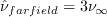
For all codes, the farfield value of the Spalart turbulence variable is
,
while CFL3D used clipping method "c" (see Note 1 on
the Spalart-Allmaras equation page).
For all codes, the farfield value of the Spalart turbulence variable is
 .
In all codes the Prandtl number Pr is taken to be constant at 0.72, and turbulent Prandtl
number Prt is taken to be constant at 0.9.
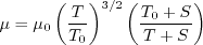
The dynamic viscosity is computed using
Sutherland's Law (See White, F. M., "Viscous Fluid Flow," McGraw Hill, New York, 1974, p. 28).
In Sutherland's Law, the local value of dynamic viscosity is determined by plugging the local value of temperature
(T) into the following formula:
.
In all codes the Prandtl number Pr is taken to be constant at 0.72, and turbulent Prandtl
number Prt is taken to be constant at 0.9.
The dynamic viscosity is computed using
Sutherland's Law (See White, F. M., "Viscous Fluid Flow," McGraw Hill, New York, 1974, p. 28).
In Sutherland's Law, the local value of dynamic viscosity is determined by plugging the local value of temperature
(T) into the following formula:
where
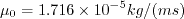 ,
,
 , and
, and
 .
The same formula can be found online
(with temperature constants given in degrees K and some small conversion differences).
Note that in terms of the reference quantities for this particular case, Sutherland's Law can equivalently be written:
.
The same formula can be found online
(with temperature constants given in degrees K and some small conversion differences).
Note that in terms of the reference quantities for this particular case, Sutherland's Law can equivalently be written:
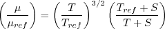
where
 is the reference dynamic viscosity that corresponds to the freestream in this case, and
freestream
is the reference dynamic viscosity that corresponds to the freestream in this case, and
freestream  is 540R. This latter form may be more convenient for nondimensional codes.
(Specific details regarding an implementation of Sutherland's Law in nondimensional codes can be found in
handwritten notes describing Sutherland's Law in CFL3D and FUN3D.)
is 540R. This latter form may be more convenient for nondimensional codes.
(Specific details regarding an implementation of Sutherland's Law in nondimensional codes can be found in
handwritten notes describing Sutherland's Law in CFL3D and FUN3D.)
Note that FUN3D and USM3D both ran this
case with first order spatial accuracy on the turbulence advection term, whereas CFL3D used second order.
It is also important to note that
unlike most other test cases on the Turbulence Modeling Resource website,
for this particular test case the structured and unstructured grids
were created independently of one another. Thus they are not related, other than the fact that the body
shape and exit plane are the same.
In particular, the outer boundary extents are different: for the structured grid, it is located
approximately 20 unit lengths from the body; whereas for the unstructured grid, it is located
approximately 10 unit lengths from the body. The grid differences may have some impact on the results.
Grid Convergence Behavior of Drag and Maximum Eddy Viscosity
Plots are shown to illustrate grid convergence for the drag coefficients and maximum eddy viscosity in the field
(the contributions to the drag coefficient due to the viscosity and pressure are presented separately).
Recall that all models were run using SA-neg.
The codes appear to be consistent for the drag values, but do not appear to be approaching the same
level for maximum eddy viscosity. The reason for this inconsistency is not known.
These plots draw attention to the fact that the
structured grids (used by CFL3D) are considerably coarser than the unstructured grids (used by FUN3D and USM3D).
For computing forces, the reference area of this case is taken to be 10 in2 (for the full 360 degrees), or
5 in2 (for a half-plane computation of 180 degrees).
Results that generated the above plots can be found in the following data files:
fun3d_drag_mut_convergence_sa.dat,
usm3d_drag_mut_convergence_sa.dat,
cfl3d_drag_mut_convergence_sa.dat.
Grid Convergence Behavior of Cp
The first plot below shows grid convergence of surface Cp at three x-locations on the body: x=0.25, x=0.5,
and x=1.50. When plotted at this scale, results look reasonably close between the three codes.
However, when zoomed in, there are differences at x=1.5 (see second plot below). The reason
for this difference is believed to primarily be the fact that the structured grid (used by CFL3D) has a farfield
extent of approximately 20 unit lengths, whereas the unstructured grid (used by FUN3D and USM3D)
has a smaller farfield extent of 10 unit lengths.


Results that generated the above plots can be found in the following data files:
fun3d_cp_convergence_sa.dat,
usm3d_cp_convergence_sa.dat,
cfl3d_cp_convergence_sa.dat.
To test the hypothesis that the farfield extent/shape has an influence on the
solution, some limited results were obtained with all 3 codes on the same grids.
The first plot below shows the FUN3D and USM3D Cp results on the default unstructured grids at
x=1.5 (these are the same results already shown above, with FF=10). Then, the second plot shows
results for all 3 codes on the default structured grids (FF=20) used by CFL3D in the
results shown above. Finally, a new set of structured grids was created with FF=10, and the 3 codes
produced the results shown in the third figure below.
Two conclusions can be made from this assessment: (1) the codes all approach the same results when run
on the same grid, and (2) the farfield boundary has an impact on the Cp at this location.
The pressure coefficient computed on the structured-grid domain with the
farfield extent of 20 converges to a value about 2.5% lower (larger in magnitude)
than the pressure coefficient computed on the structured domain with the farfield extent of 10.
There is also apparently
a sensitivity to the shape of the farfield boundary when located in a relatively close proximity to the surface: the
pressure coefficients computed on domains with similar locations and different shapes of the farfield boundaries differ
by about 1.3% (compare the 2 results with FF=10).
Results that generated the above plots can be found in the following data files:
fun3d_cp_convergence_sa_str_grids.dat,
usm3d_cp_convergence_sa_str_grids.dat,
cfl3d_cp_convergence_sa_str_grids.dat.
Cp and Cf Axially
The Cp and Cf distributions (axially, on the body)
from the three codes on the finest grid are shown in the following figures. All
results are very close to plotting accuracy.


Results that generated the above Cp plots can be found in the following data files:
fun3d_cp_axial_sa.dat,
usm3d_cp_axial_sa.dat,
cfl3d_cp_axial_sa.dat.
Results that generated the above Cf plots can be found in the following data files:
fun3d_cf_axial_sa.dat,
usm3d_cf_axial_sa.dat,
cfl3d_cf_axial_sa.dat.
Cp, U-Velocity, and Eddy Viscosity Along a Spanwise Grid Line
The following plots show Cp and u-velocity along a radial line emanating from the surface at x=0.5:


Results that generated the above plots can be found in the following data files:
fun3d_various_radial_sa.dat,
usm3d_various_radial_sa.dat,
cfl3d_various_radial_sa.dat.
The following plot shows eddy viscosity along the same radial line emanating from the surface at x=0.5:

Results that generated the above plots can be found in the following data files:
fun3d_mut_radial_sa.dat,
usm3d_mut_radial_sa.dat,
cfl3d_mut_radial_sa.dat.
Radial Variations on the Surface
The following plots show radial variations of Cp and Cf at the location x=0.25, using 3 grid levels.
There is very little circumferential variation in the structured-grid CFL3D results, but on the unstructured grids
both FUN3D and USM3D show variations, particularly near the boundaries of 60-degree sectors, where
there are abrupt changes in the surface grid triangulation.
Results that generated the above plots can be found in the following data files:
fun3d_cp_circum_sa.dat,
usm3d_cp_circum_sa.dat,
cfl3d_cp_circum_sa.dat.
Results that generated the above plots can be found in the following data files:
fun3d_cf_circum_sa.dat,
usm3d_cf_circum_sa.dat,
cfl3d_cf_circum_sa.dat.
Return to: 3D Hemisphere Cylinder Validation for Numerical Analysis Intro Page
Return to: Turbulence Modeling Resource Home Page
Privacy Act Statement
Accessibility Statement
Responsible NASA Official:
Ethan Vogel
Page Curator:
Clark Pederson
Last Updated: 11/05/2021


