Langley Research Center Turbulence Modeling Resource

 

Jump to: SA Results,  SA-RC Results,  SSTm Results,  SST-RCm Results,  SSG/LRR-RSM-w2012 Results,  Wilcox2006-klim-m Results,  EASMko2003-S Results,  K-e-Rt-RC Results

Return to: 2D Convex Curvature Boundary Layer Case Intro Page

Return to: Turbulence Modeling Resource Home Page

2D Convex Curvature Boundary Layer Validation Case

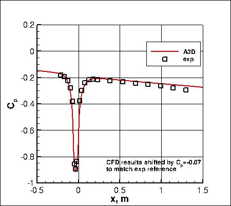
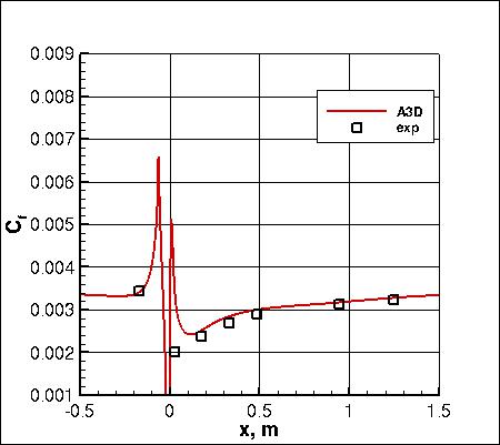
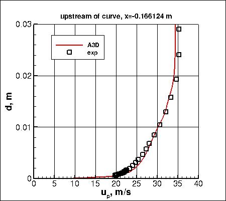
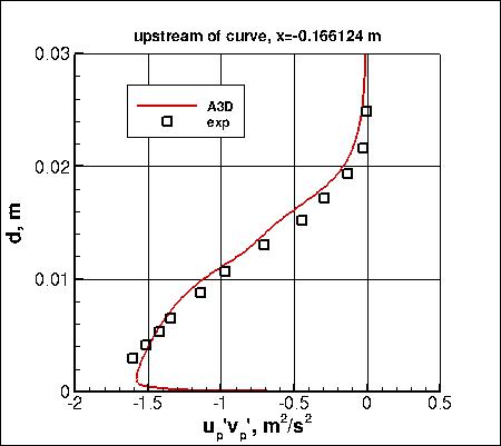
GLVY-RSM-2012 Model Results
 

Link to GLVY-RSM-2012 equations

Note that thorough grid studies were not performed for validation cases such as this one. Some effort was made to ensure reasonable grid resolutions, but there may still be small noticeable discretization errors. Therefore, these validation results shown should be considered representative, but not "truth."

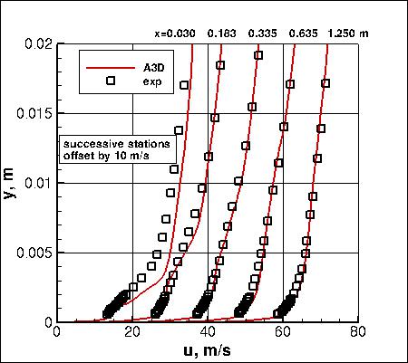
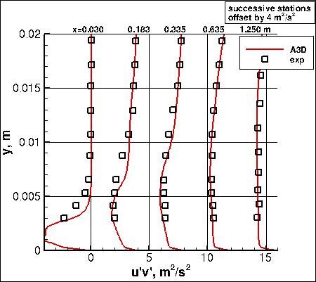
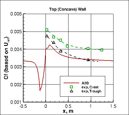
Above GLVY-RSM-2012 results are from the code aerodynamics.1.0.3 on the 1025x385 grid. The inflow boundary-layer thickness was 0.0005 m = 0.5 mm (the computations were also run with no boundary layer imposed at the inflow, and very similar results were obtained). The inflow turbulence intensity = 1% and freestream lengthscale = 0.125 m = 125 mm, which is roughly the duct's height (see Note 4 on GLVY model description page). The other computational parameters and post-processing to get the local velocities and Reynolds-stresses in the wall-aligned frame are those of the test-case description (see 2D Convex Curvature Boundary Layer Case Intro Page). For the station at x=-0.166124 m, the parallel velocity component u_p is the velocity parallel to the wall (which is canted at 30 deg relative to Cartesian coordinates), and the u_p'v_p' is taken with respect to the wall-normal and wall-parallel directions. The formulas for computing these rotated quantities from Cartesian quantities are:

• u_p = u*cos(theta) + v*sin(theta)
• u_p'v_p' = 0.5*(v'v'-u'u')*sin(2*theta) + u'v'*cos(2*theta)

Although the main focus of this case is on the bottom (convex) wall region, top (concave) wall skin friction results from the 2-D computation are also shown in the last plot above.

Data files from A3D are given here for reference: smits_cp_A3D_GLVY.dat, smits_cf_A3D_GLVY.dat, smits_u_upstream_A3D_GLVY.dat, smits_uv_upstream_A3D_GLVY.dat, smits_u_A3D_GLVY.dat, smits_uv_A3D_GLVY.dat, and smits_cftopwall_A3D_GLVY.dat.

Note that this model is currently assigned MRR Level 1 for the purposes of this website. This is because at this time the TMBWG has results for this model from only one code. The results on this page are therefore not necessarily reliable until additional independent code(s) can be used to verify the model implementation.

Note that the wall-shapes in the curved region have (unintentional) small oscillations in the second-derivative of the provided grids; these cause small oscillations in Cp and Cf near their peaks (not easily visible at the scales of the plots above).

Note that these are compressible code results at "essentially incompressible" conditions of M=0.093. There may be a very small influence of compressibility.
 
 

Jump to: SA Results,  SA-RC Results,  SSTm Results,  SST-RCm Results,  SSG/LRR-RSM-w2012 Results,  Wilcox2006-klim-m Results,  EASMko2003-S Results,  K-e-Rt-RC Results

Return to: 2D Convex Curvature Boundary Layer Case Intro Page

Return to: Turbulence Modeling Resource Home Page

Recent significant updates:
01/27/2015 - mention of oscillations in second derivative of wall shape in provided grids

Privacy Act Statement

Accessibility Statement

Responsible NASA Official: Ethan Vogel
Page Curator: Clark Pederson
Last Updated: 03/23/2021