Langley Research Center Turbulence Modeling Resource

 

Jump to: SA Results,  SA-RC Results,  SST-RCm Results,  SSG/LRR-RSM-w2012 Results,  Wilcox2006-klim-m Results,  EASMko2003-S Results,  K-e-Rt-RC Results,  GLVY-RSM-2012 Results

Return to: 2D Convex Curvature Boundary Layer Case Intro Page

Return to: Turbulence Modeling Resource Home Page

2D Convex Curvature Boundary Layer Validation Case

SSTm Model Results
 

Link to SSTm equations

Previously on this page the results were reported as SST solutions, but more properly they should be referred to as SSTm. Essentially no difference is expected.

Note that thorough grid studies were not performed for validation cases such as this one. Some effort was made to ensure reasonable grid resolutions, but there may still be small noticeable discretization errors. Therefore, these validation results shown should be considered representative, but not "truth."

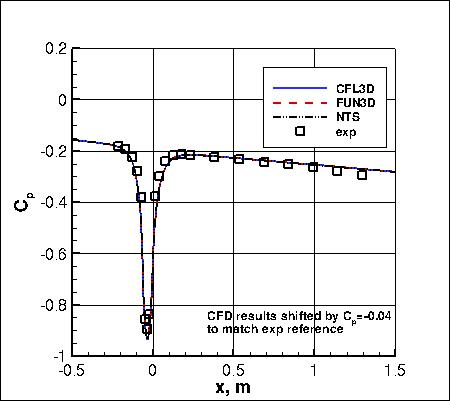
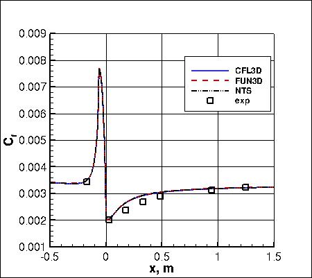
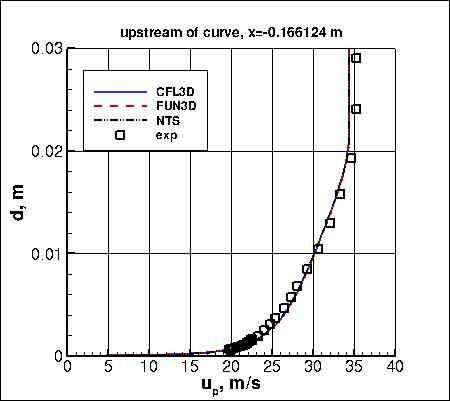
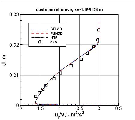
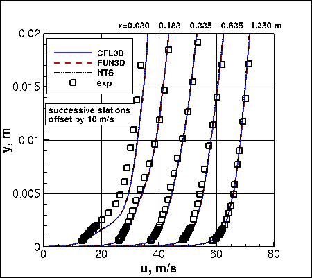
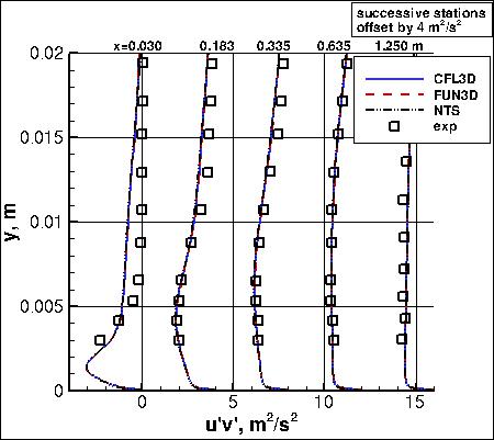
Above SSTm results are from three independent CFD codes: CFL3D and FUN3D (NASA LaRC, USA), and NTS (NTS, Russia). All three codes used freestream turbulence intensity=0.083% and freestream turbulent viscosity (relative to laminar)=0.009 (additional details can be found in the CFL3D User's Manual, Appendix H). Please read note 5 on Notes on running CFD page. They all used the same 513x193 grid. All three yield nearly identical results for all quantities. For the station at x=-0.166124 m, the parallel velocity component u_p is the velocity parallel to the wall (which is canted at 30 deg relative to Cartesian coordinates), and the u_p'v_p' is taken with respect to the wall-normal and wall-parallel directions. The formulas for computing these rotated quantities from Cartesian quantities are:

• u_p = u*cos(theta) + v*sin(theta)
• u_p'v_p' = 0.5*(v'v'-u'u')*sin(2*theta) + u'v'*cos(2*theta)

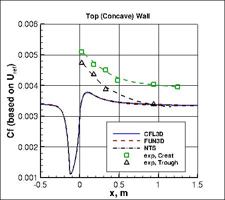
Although the main focus of this case is on the bottom (convex) wall region, top (concave) wall skin friction results from the 2-D computation are also shown in the last plot above.

Note that the wall-shapes in the curved region have (unintentional) small oscillations in the second-derivative of the provided grids; these cause small oscillations in Cp and Cf near their peaks (not easily visible at the scales of the plots above).

Note that these are compressible code results at "essentially incompressible" conditions of M=0.093. There may be a very small influence of compressibility. Only the CFD data files from CFL3D are given here for reference: smits_cp_cfl3d_sst.dat, smits_cf_cfl3d_sst.dat, smits_u_upstream_cfl3d_sst.dat, smits_uv_upstream_cfl3d_sst.dat, smits_u_cfl3d_sst.dat, smits_uv_cfl3d_sst.dat, and smits_cftopwall_cfl3d_sst.dat. A typical CFL3D input file is: smits_cfl3d_typical_sst.inp. A typical FUN3D input file is: fun3d.nml_typical_sst.

Jump to: SA Results,  SA-RC Results,  SST-RCm Results,  SSG/LRR-RSM-w2012 Results,  Wilcox2006-klim-m Results,  EASMko2003-S Results,  K-e-Rt-RC Results,  GLVY-RSM-2012 Results

Return to: 2D Convex Curvature Boundary Layer Case Intro Page

Return to: Turbulence Modeling Resource Home Page

Recent significant updates:
01/27/2015 - mention of oscillations in second derivative of wall shape in provided grids

Privacy Act Statement

Accessibility Statement

Responsible NASA Official: Ethan Vogel
Page Curator: Clark Pederson
Last Updated: 03/13/2025