The purpose here is to provide a
validation case for turbulence models. Unlike verification, which seeks to
establish that a model has been implemented correctly, validation compares
CFD results against data in an effort to establish a model's ability to
reproduce physics. A large sequence of nested grids of the same family are
provided here if desired. Data are also provided for comparison. For this
particular "essentially incompressible" curvature
case (from Smits, Young, and Bradshaw), the data are from experiments.
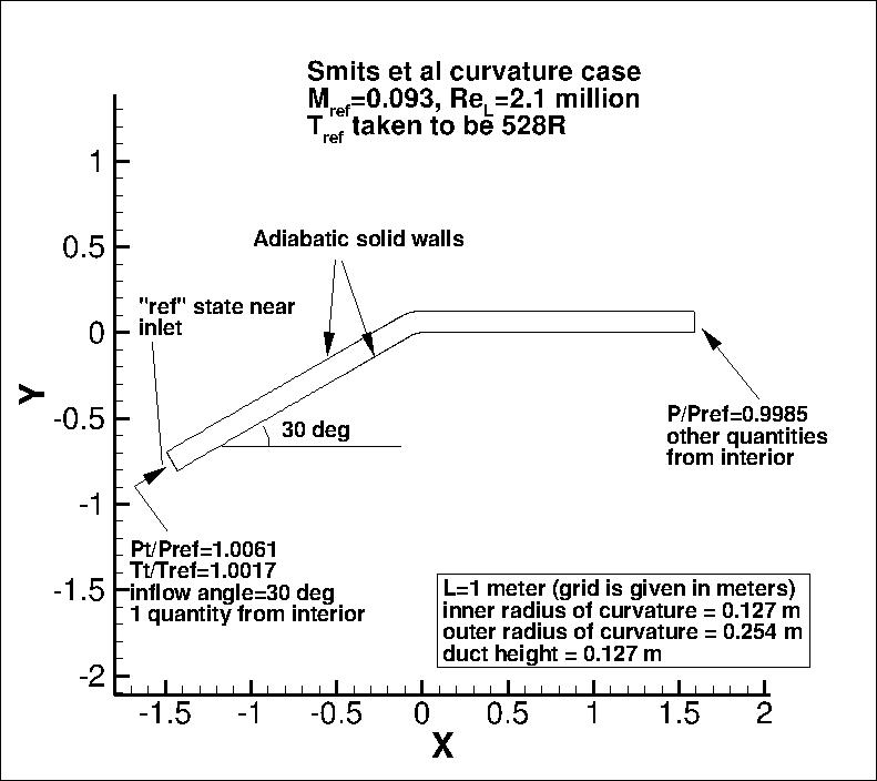
The experiment utilizes a constant area square duct of height 0.127 m with a rapid 30 degree bend
(inner radius of curvature is 0.127 m). In the experiment, the aspect ratio of the duct was 6:1.
The primary focus of this case is to assess turbulence models for convex wall curvature
(the lower wall in this case).
Near convex walls, turbulence levels are known to decrease in comparison to flow near
straight walls. Here, different models are
assessed in their ability to capture this effect.
(Note that this case also has an upper (concave) wall, where the opposite occurs.
The concave wall destabilizes boundary layers, increasing turbulence levels and the thickness of
the boundary layer. In concave curvature, Gortler vortices generally form. These vortices tend
to be quasi-stable, and can result in steady or slowly varying, large scale spanwise variations
in boundary layer. Although not the primary focus of this case,
the measurements from the Smits case on the concave wall show significant
spanwise variations in the skin friction, consistent with the presence of Gortler vortices.
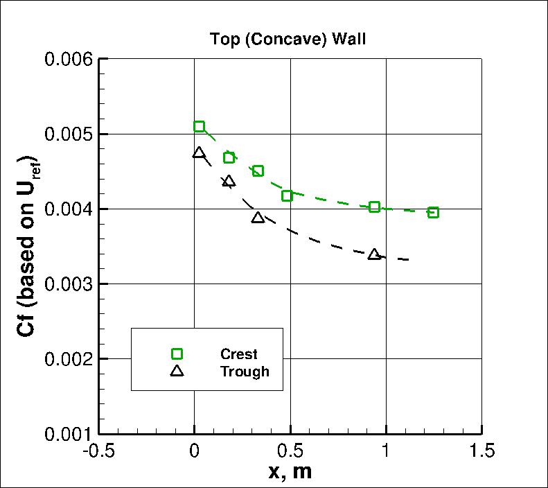
We provide curves for the minimum and maximum skin friction along the concave wall from the
test. Given the nature of streamwise flow in concave curvature,
interpretations of differences between CFD and test in this region should take into account
both the uncertainty in the test results and the difficulty of capturing Gortler vortices
in a steady state computation in 3-D, and the impossibility of capturing their effects
in 2-D. For this test case the duct is modeled in 2-D.
Results on the concave wall are provided for guidance and comparison between models,
but should not be interpreted as a definitive discriminator between models.)
The reference velocity (Uref) near the inlet is 31.9 m/s.
The back pressure is chosen to achieve the desired flow. The upstream
"run" length is chosen to allow the fully turbulent boundary layer
to develop naturally, and achieve approximately the correct boundary layer thickness
upstream of the bend. The upper
and lower boundaries are modeled as adiabatic solid walls.
The following plot shows the layout of this case, along with the boundary conditions.
"Pt" refers to total pressure, "P" refers to
static pressure, and "Tt" refers to total temperature.
GRIDS
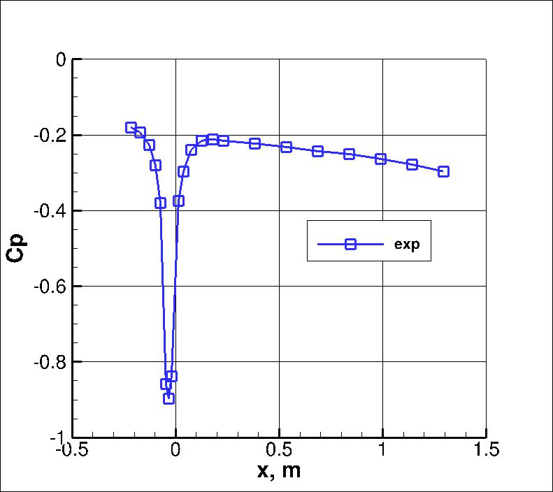
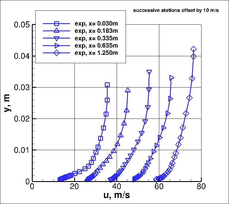
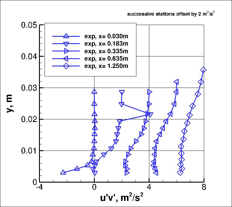
Some of the experimental data for this case will be shown below.
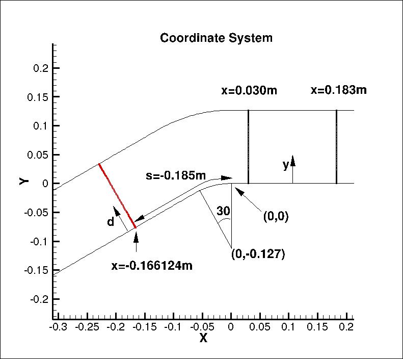
The profiles of interest are at s= -0.185 m (x=-0.166124 m) upstream of the bend, and
x= 0.030, 0.183, 0.335, 0.635, and 1.250 downstream of the bend.
Data are given in local coordinates aligned with the inner duct wall and wall normal.
The experimental data reference is: Smits, A. J., Young, S. T. B., Bradshaw, P.
"The Effect of Short Regions of High Surface Curvature on Turbulent Boundary Layers,"
J. Fluid Mech., Vol. 94, Part 2, 1979, pp. 209-242,
https://doi.org/10.1017/S0022112079001002.
The experimental data are available on this site from:
Note that some inconsistencies were discovered in the experimental data
as posted from Oct 30, 1981, in comparison with JFM (1979). The data were
revisited with the help of the original author (Lex Smits) during
Oct-Nov 2012. The corrected data are provided.
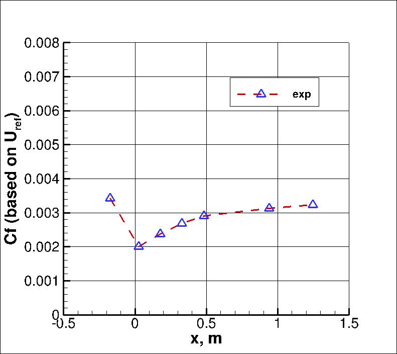
Note that skin friction coefficient values are given here based on Uref, for
convenience when comparing against CFD results. However, the original experimental data files
give Cf based on local edge velocity Ue.
In the above plots, the s locations have been translated to x for s less than -0.066497.
The three points on the Cp curve lying between s=-0.066497 and s=0 simply plot s rather than x
(for convenience); visually it makes no noticeable difference.
Note that the Cf experimental data are very sparse; they miss a dramatic localized
increase that occurs between x=-0.2 and x=0 m.
The main focus of this case is the region near the bottom (convex) wall.
Data near the top (concave) wall were not provided in the on-line dataset F-0235. However, the journal
article provides some information. For example, the following plot shows a range of concave
wall skin friction coefficients (nondimensionalized by Uref), as measured at approximate "crest" and
"trough" locations. It is well-known that concave
curvature tends to be very three-dimensional (with
Gortler vortices).
The experimental data for this plot can be found in the following file:
cf_concaveside_final.dat.
What to Expect:
(Other turbulence model results may be added in the future.)
Note that the OVERFLOW code has documented its results for this validation case (for the SA-noft2, SA-noft2-RC, SST, and SST-RC
turbulence models) in NAS Technical Paper 2016-01 (pdf file)
(18.3 MB) by Jespersen, Pulliam, and Childs.
Return to: Turbulence Modeling Resource Home Page
Recent significant updates:
03/31/2020 - better clarification between convex and concave curvature in discussion
03/24/2015 - added link to SST-RC results
Privacy Act Statement
Accessibility Statement
Responsible NASA Official:
Ethan Vogel
Page Curator:
Clark Pederson
Last Updated: 11/18/2021

