Langley Research Center

Turbulence Modeling Resource

Return to: Turbulence Modeling Resource Home Page

2DZP: 2D Zero Pressure Gradient Flat Plate Validation Case

The purpose here is to provide a validation case for turbulence models. Unlike verification, which seeks to establish that a model has been implemented correctly, validation compares CFD results against data in an effort to establish a model's ability to reproduce physics. A large sequence of nested grids of the same family are provided here if desired. Data are also provided for comparison. For this particular "essentially incompressible" flat plate case, the data are from theory. This case is the same case used for Flat Plate Verification; however, for the purpose of validation here, different quantities of interest are focused on and compared.

The turbulent flat plate case should be run at essentially incompressible conditions (for example, M = 0.2 or less in compressible CFD codes). For the grids given below, running at a Reynolds number per unit length of Re = 5 million is sufficient to achieve desired Re_theta levels. The following plot shows the layout of the simple flat plate grids, along with typical boundary conditions. (Note that particular variations of the BCs at the inflow, top wall, and outflow may also work and yield similar results for this problem.)

Note that for this case the maximum boundary layer thickness is about 0.03 L, so the grid height of y=L is far enough away to have very little influence. For example, a test in which the upper extent was moved down to y=0.48 L only changed results (integrated drag or skin friction at x=0.97) by less than 0.2%.

Grids are provided below. Note that different turbulence models exhibit different sensitivities to minimum wall-normal spacing.
flat plate grid layout & BCs

GRIDS (same as those used for Flat Plate Verification case)

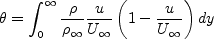
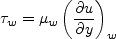
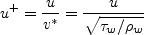
Two quantities of interest are desired for comparison:

Wall skin friction coefficient vs. Re_theta (for 4000 < Re_theta < 13,000)
u+ vs. y+ (at Re_theta=10,000)

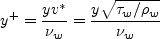
Definitions are given here for the relevant quantities, including Re_theta, Cf, u+, and y+

$Re_{\theta} = \frac{\rho_{\infty} U_{\infty} \theta}{\mu_{\infty}}$

$\theta = \int_0^{\infty} \frac{\rho}{\rho_{\infty}} \frac{u}{U_{\infty}} \left( 1 - \frac{u}{U_{\infty}} \right) dy$

$c_f = \frac{\tau_w}{\frac{1}{2} \rho_{\infty} U_{\infty}^2}$

$\tau_w = \mu_w \left( \frac{\partial u}{\partial y} \right)_w$

$u^+ = \frac{u}{v^*} = \frac{u}{\sqrt{\tau_w / \rho_w}}$

$y^+ = \frac{y v^*}{\nu_w} = \frac{y \sqrt{\tau_w / \rho_w}}{\nu_w}$

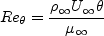
It should be noted that computing Re_theta typically involves an additional post-processing step for many CFD codes (numerically integrating to obtain theta). Although this step is relatively straightforward for the flat plate, nonetheless some numerical errors are unavoidably introduced which may vary depending on the postprocessing program employed. When viewing comparisons, this additonal potential source of error should be taken into consideration.

The following plot shows Re_theta as a function of x for this flat plate case, from a variety of different turbulence models. Clearly, the particular model makes some difference, but the general trend can be discerned: Re_theta increases from near zero at the plate leading edge to somewhat over 14,000 at x=2.
Re_theta as function of x for flat plate case

A data file with a typical variation of Re_theta as function of x is given here: retheta_variation_typical.dat.

Theoretical curves for comparison are given below. For wall skin friction comparison, the Karman-Schoenherr (K-S) relation (Schoenherr, K. E., Trans. SNAME. 40:279-313, 1932) is used:

$c_f = \left( 17.08 \left({\rm log}_{10}Re_{\theta} \right)^2 + 25.11 \left( {\rm log}_{10}Re_{\theta} \right) + 6.012 \right)^{-1}$

For u+ vs. y+, the law-of-the-wall based on Coles' mean velocity profile (Coles, D., J. Fluid Mech. 1(2):191-226, 1956, https://doi.org/10.1017/S0022112056000135 and Coles, D., RAND Corp Rept. R-403-PR, 1962, https://www.rand.org/pubs/reports/R403.html) is used

$u^+ = \frac{1}{\kappa} {\rm ln} \left( y^+ \right) + C + \frac{2 \Pi}{\kappa} \left[ {\rm sin} \left( \frac{\pi y}{2 \delta} \right) \right]^2$

along with a van Driest type damping near the wall. A program provided by P. G. Huang was used to compute these mean profiles. See Bardina et al, NASA TM 110446, April 1997, https://ntrs.nasa.gov/citations/19970017828 for more details. The data files for these correlations are provided here:

Note that these particular theoretical correlations are not necessarily perfect. There is some uncertainty in trying to match a wide range of experimental data. Results from these correlations alongside other theories (from White, F. M., "Viscous Fluid Flow," McGraw Hill, New York, 1974) are plotted in the following figures:
other skin friction correlations
other similarity laws

White ("Viscous Fluid Flow," McGraw Hill, New York, 1974) also provides various theories for flat plate Cf as a function of Re_x (for example, see equations 6-112a, 6-121, and 6-134 in that reference). For the current case of Re_L=5 million (L=2), these equations can be plotted as a function of x, as follows (note that error bars of 5% have been included although it is not clear what the error levels actually are):
Cf theories as function of x for current case

Like the earlier plot of Cf vs Re_theta, this plot provides a feel for the approximate theoretical range of wall skin friction coefficients for this case. The data file that produced the above plot is: cf_as_function_of_x.dat.

What to Expect:

RESULTS
LINK TO EQUATIONS
MRR Level

SA
SA eqns
4

SSTm
SSTm eqns
3

SST-Vm
SST-Vm eqns
3

BSLm
BSLm eqns
2

SSG/LRR-RSM-w2012
SSG/LRR-RSM-w2012 eqns
3

Wilcox2006-klim-m
Wilcox2006-klim-m eqns
2

K-kL-MEAH2015m
K-kL-MEAH2015m eqns
3

EASMko2003-S
EASMko2003-S eqns
1

K-e-Rt
K-e-Rt eqns
1

GLVY-RSM-2012
GLVY-RSM-2012 eqns
1

(Other turbulence model results may be added in the future.)

Note that the OVERFLOW code has documented its results for this validation case (for the SA-noft2, SST, and SST-V turbulence models) in NAS Technical Paper 2016-01 (pdf file) (18.3 MB) by Jespersen, Pulliam, and Childs.

Return to: Turbulence Modeling Resource Home Page

Recent significant updates:
04/12/2022 - added plot of theoretical Cf vs x and provided data file
08/28/2020 - changed SST-V naming to SST-Vm
11/07/2017 - added link to discussion on effect of minimum wall-normal grid spacing
05/13/2016 - added BSL link
06/16/2016 - changed K-kL-MEAH2013 to K-kL-MEAH2015
08/20/2014 - added SSG/LRR-RSM-w2012 link
06/23/2014 - added typical variation of Re_theta with x for this case

Privacy Act Statement

Accessibility Statement

Responsible NASA Official: Ethan Vogel
Page Curator: Clark Pederson
Last Updated: 04/12/2022

RESULTS	LINK TO EQUATIONS	MRR Level
SA	SA eqns	4
SSTm	SSTm eqns	3
SST-Vm	SST-Vm eqns	3
BSLm	BSLm eqns	2
SSG/LRR-RSM-w2012	SSG/LRR-RSM-w2012 eqns	3
Wilcox2006-klim-m	Wilcox2006-klim-m eqns	2
K-kL-MEAH2015m	K-kL-MEAH2015m eqns	3
EASMko2003-S	EASMko2003-S eqns	1
K-e-Rt	K-e-Rt eqns	1
GLVY-RSM-2012	GLVY-RSM-2012 eqns	1